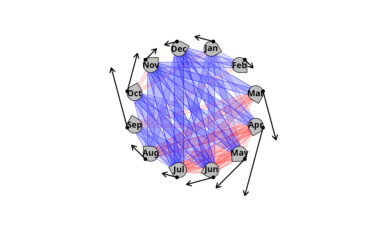
Adds arrows representing cyclical shifts (advances/delays) into convergence/divergence plots created using function trajectoryConvergencePlot.
Usage
cycleShiftArrows(
  cycle.shifts,
  radius = 1,
  top = "between",
  cycle.shifts.inf.conf = NULL,
  cycle.shifts.sup.conf = NULL,
  arrows.length.mult = "auto",
  arrows.lwd = 2
)
Arguments
- cycle.shifts
Cyclical shifts computed for each fixed date trajectory plotted by
trajectoryConvergencePlot.- radius
The radius of the circles representing trajectories. Defaults to 1.
- top
A string indicating if the top of the plotting area should contain a circle representing a trajectory ("circle"), or should be in between two circles ("between"). Defaults to "between".
- cycle.shifts.inf.conf
Lower confidence intervals for cyclical shifts.
- cycle.shifts.sup.conf
Upper confidence intervals for cyclical shifts.
- arrows.length.mult
A multiplication coefficient for the arrows representing cyclical shifts. Attempts an automatic adjustment by default (dividing by max(cycle.shifts)).
- arrows.lwd
Line width of the arrows. Defaults to 2.
Details
This function is meant to be used in conjunction with trajectoryConvergencePlot, to study fixed-date trajectories convergence/divergence patterns:
First, setting
pointy = TRUE, in the call totrajectoryConvergencePlot, when the studied trajectories are the outputs ofextractFixedDateTrajectoriesallows to suggest cyclicity.Second, function
cycleShiftArrowsallows to represent cyclical shifts by adding arrows to the circles representing trajectories. Clockwise arrows will represent advances, anticlockwise arrows will represent delays. Arrows length is proportional to the cyclical shift provided. Relevant measures of cyclical shifts have to be computed by the user. A variety of methods may be employed but the outputs ofcycleShiftscannot be used immediately as they do not directly correspond to the fixed-date trajectories. An example of how to compute relevant measures of cyclical shifts is provided incycleShiftsand in the CETA vignette. The argumentsradiusandtopincycleShiftArrowsmust match those in the corresponding call totrajectoryConvergencePlotfor proper display.
Examples
# \donttest{
#Load cyclical data (a monthly resolved long-term time series of north sea zooplankton)
data("northseaZoo")

#Define trajectories
traj <- defineTrajectories(d = dist(northseaZoo$Hellinger),
                           times = northseaZoo$times,
                           sites = northseaZoo$sites)

#Simplify it using only one site
traj <- subsetTrajectories(traj, site_selection = "NNS")

#Extract the fixed date trajectories
fdT <- extractFixedDateTrajectories(traj, cycleDuration = 1)

#Make the convergence/divergence plot
trajectoryConvergencePlot(fdT,
                         type = "pairwise.symmetric",
                         radius = 1.2,
                         alpha.filter = 0.05,
                         half.arrows.size = 2,
                         pointy = TRUE,
                         traj.names = c("Jan", "Feb", "Mar", "Apr", "May", "Jun",
                                        "Jul", "Aug", "Sep", "Oct", "Nov", "Dec"))

#Compute the cyclical shifts (this takes a bit of time)
CS <- cycleShifts(traj, cycleDuration = 1)

#Obtain an average cyclical shift for each month (this is not automated by ecotraj,
#since many ways to do it can be justified). Here we obtain it as the slope of the regression
#line of cyclical shifts (y) on the corresponding time scale (x).
averageCS <- integer(0)
for (i in unique(CS$dateCS)){
  CSmonth <- CS[CS$dateCS==i,]
  model <- lm(CSmonth$cyclicalShift~CSmonth$timeScale)
  averageCS <- c(averageCS,model$coefficients[2])
}

#Add the average cyclical shifts to the plot
cycleShiftArrows(averageCS, radius = 1.2)


# }
# }