Functions to compare pairs of trajectories or trajectory segments.
Function
segmentDistancescalculates the distance between pairs of trajectory segments.Function
trajectoryDistancescalculates the distance between pairs of trajectories.Function
trajectoryConvergenceperforms the Mann-Kendall trend test on (1) the distances between trajectories; (2) the distance between points of one trajectory to the other; or (3) the variance of states among trajectories.Function
trajectoryCorrespondenceperforms a permutation test of pairwise dynamic correspondence between trajectories sensitive to trajectory shape and movement direction.Function
trajectoryShiftscalculates trajectory shifts (i.e. advances and delays) between trajectories assumed to follow a similar path but with different speeds or time lags.
Usage
segmentDistances(x, distance.type = "directed-segment", add = TRUE)

trajectoryDistances(
  x,
  distance.type = "DSPD",
  symmetrization = "mean",
  add = TRUE
)

trajectoryConvergence(x, type = "pairwise.asymmetric", add = TRUE)

trajectoryCorrespondence(x, nperm = 999, verbose = FALSE)

trajectoryShifts(x, add = TRUE)
Arguments
- x
An object of class
trajectories.- distance.type
The type of distance index to be calculated (see section Details).
- add
Flag to indicate that constant values should be added (local transformation) to correct triplets of distance values that do not fulfill the triangle inequality.
- symmetrization
Function used to obtain a symmetric distance, so that DSPD(T1,T2) = DSPD(T2,T1) (e.g.,
mean,maxormin). Ifsymmetrization = NULLthen the symmetrization is not conducted and the output dissimilarity matrix is not symmetric.- type
A string indicating the convergence test, either
"pairwise.asymmetric","pairwise.symmetric"or"multiple"(see details).- nperm
The number of permutations to be used in the dynamic correspondence test. Defaults to
999.- verbose
Boolean. Should the function indicate its progress? Useful to estimate computing time if many comparisons are performed. Defaults to
FALSE.
Value
Function trajectoryDistances returns an object of class dist containing the distances between trajectories (if symmetrization = NULL then the object returned is of class matrix).
Function segmentDistances list with the following elements:
Dseg: Distance matrix between segments.Dini: Distance matrix between initial points of segments.Dfin: Distance matrix between final points of segments.Dinifin: Distance matrix between initial points of one segment and the final point of the other.Dfinini: Distance matrix between final points of one segment and the initial point of the other.
Function trajectoryConvergence returns a list with two elements:
tau: A single value or a matrix with the statistic (Mann-Kendall's tau) of the convergence/divergence test between trajectories. Iftype = "pairwise.symmetric"then the matrix is square and iftype = "pairwise.asymmetric"the statistic of the test of the row trajectory approaching the column trajectory. Iftype = "multiple"tau is a single value.p.value: A single value or a matrix with the p-value of the convergence/divergence test between trajectories. Iftype = "pairwise.symmetric"then the matrix of p-values is square and iftype = "pairwise.asymmetric"then the p-value indicates the test of the row trajectory approaching the column trajectory. Iftype = "multiple"p-value is a single value.
Function trajectoryCorrespondence returns a square matrix with permutation p-values in the lower triangle and the test statistics in the upper triangle.
Function trajectoryShifts returns an object of class data.frame describing trajectory shifts (i.e. advances and delays). The columns of the data.frame are:
reference: the site (trajectory) that is taken as reference for shift evaluation.site: the target site (trajectory) for which shifts have been computed.survey: the target trajectory survey for which shift is computed.time: the time corresponding to target trajectory survey.timeRef: the time associated to the projected ecological state onto the reference trajectory.shift: the time difference between the time of the target survey and the time of projected ecological state onto the reference trajectory. Positive values mean faster trajectories and negative values mean slower trajectories.
Details
Ecological Trajectory Analysis (ETA) is a framework to analyze dynamics of ecological entities described as trajectories in a chosen space of multivariate resemblance (De Cáceres et al. 2019). ETA takes trajectories as objects to be analyzed and compared geometrically.
The input distance matrix d should ideally be metric. That is, all subsets of distance triplets should fulfill the triangle inequality (see utility function is.metric).
All ETA functions that require metricity include a parameter 'add', which by default is TRUE, meaning that whenever the triangle inequality is broken the minimum constant required to fulfill it is added to the three distances.
If such local (an hence, inconsistent across triplets) corrections are not desired, users should find another way modify d to achieve metricity, such as PCoA, metric MDS or non-metric MDS (see vignette 'Introduction to Ecological Trajectory Analysis').
If parameter 'add' is set to FALSE and problems of triangle inequality exist, ETA functions may provide missing values in some cases where they should not.
The resemblance between trajectories is done by adapting concepts and procedures used for the analysis of trajectories in space (i.e. movement data) (Besse et al. 2016).
Parameter distance.type is the type of distance index to be calculated which for function segmentDistances has the following options (Besse et al. 2016, De Cáceres et al. 2019):
Hausdorff: Hausdorff distance between two segments.directed-segment: Directed segment distance (default).PPA: Perpendicular-parallel-angle distance.
In the case of function trajectoryDistances the following values are possible (De Cáceres et al. 2019):
Hausdorff: Hausdorff distance between two trajectories.SPD: Segment Path Distance.DSPD: Directed Segment Path Distance (default).TSPD: Time-Sensitive Path Distance (experimental).
When using trajectoryDistances on trajectory cycles, then the elements to be compared are cycles. In this case, if TSPD is used the time of the first survey is subtracted to all times of the cycle, so that cycle dates are effectively used.
Function trajectoryConvergence is used to study convergence/divergence between trajectories. There are three possible tests, the first two concerning pairwise comparisons between trajectories.
If
type = "pairwise.asymmetric"then all pairwise comparisons are considered and the test is asymmetric, meaning that we test for trajectory A approaching trajectory B along time. This test uses distances of orthogonal projections (i.e. rejections) of states of one trajectory onto the other.If
type = "pairwise.symmetric"then all pairwise comparisons are considered but we test whether the two trajectories become closer along surveys. This test requires the same number of surveys for all trajectories and uses the sequence of distances between states of the two trajectories corresponding to the same survey.If
type = "multiple"then the function performs a single test of convergence among all trajectories. This test needs trajectories to be synchronous. In this case, the test uses the sequence of variability between states corresponding to the same time.
In all cases, a Mann-Kendall test (see cor.test) is used to determine if the sequence of values is monotonously increasing or decreasing. Function trajectoryConvergencePlot provides options for plotting convergence/divergence between trajectories.
Function trajectoryCorrespondence is used to study the dynamic correspondence between pairs of trajectories (Djeghri et al. in prep) sensitive to trajectory shape and direction of movement.
The function performs a permutation test with a positive test statistic indicative of similar movement direction whereas a negative test statistic indicates trajectories going in opposed directions.
This test requires the same numbers of surveys for all trajectories.
Function trajectoryShifts is intended to be used to compare trajectories that are assumed to follow a similar pathway. The function
evaluates shifts (advances or delays) due to different trajectory speeds or the existence of time lags between them. This is done using calls to trajectoryProjection.
Whenever the projection of a given target state on the reference trajectory does not exist the shift cannot be evaluated (missing values are returned).
References
Besse, P., Guillouet, B., Loubes, J.-M. & François, R. (2016). Review and perspective for distance based trajectory clustering. IEEE Trans. Intell. Transp. Syst., 17, 3306–3317.
De Cáceres M, Coll L, Legendre P, Allen RB, Wiser SK, Fortin MJ, Condit R & Hubbell S. (2019). Trajectory analysis in community ecology. Ecological Monographs 89, e01350.
Djeghri et al. (in preparation) Uncovering the relative movements of ecological trajectories.
Examples
#Description of entities (sites) and surveys
entities <- c("1","1","1","1","2","2","2","2","3","3","3","3")
surveys <- c(1,2,3,4,1,2,3,4,1,2,3,4)
#Raw data table
xy<-matrix(0, nrow=12, ncol=2)
xy[2,2]<-1
xy[3,2]<-2
xy[4,2]<-3
xy[5:6,2] <- xy[1:2,2]
xy[7,2]<-1.5
xy[8,2]<-2.0
xy[5:6,1] <- 0.25
xy[7,1]<-0.5
xy[8,1]<-1.0
xy[9:10,1] <- xy[5:6,1]+0.25
xy[11,1] <- 1.0
xy[12,1] <-1.5
xy[9:10,2] <- xy[5:6,2]
xy[11:12,2]<-c(1.25,1.0)
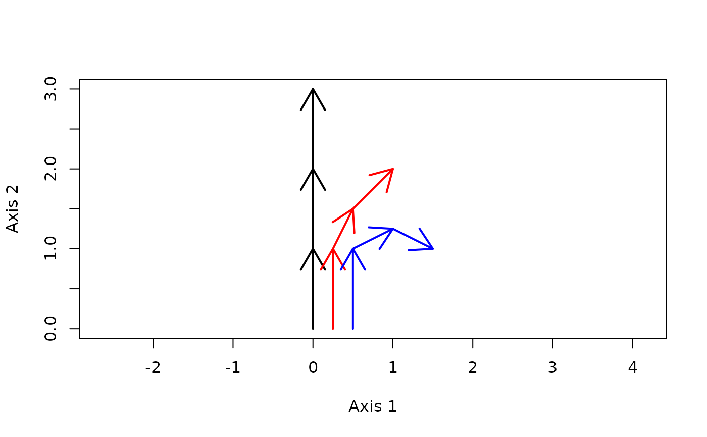
#Draw trajectories
trajectoryPlot(xy, entities, surveys,
traj.colors = c("black","red", "blue"), lwd = 2)
 #Distance matrix
d <- dist(xy)
d
#> 1 2 3 4 5 6 7
#> 2 1.0000000
#> 3 2.0000000 1.0000000
#> 4 3.0000000 2.0000000 1.0000000
#> 5 0.2500000 1.0307764 2.0155644 3.0103986
#> 6 1.0307764 0.2500000 1.0307764 2.0155644 1.0000000
#> 7 1.5811388 0.7071068 0.7071068 1.5811388 1.5206906 0.5590170
#> 8 2.2360680 1.4142136 1.0000000 1.4142136 2.1360009 1.2500000 0.7071068
#> 9 0.5000000 1.1180340 2.0615528 3.0413813 0.2500000 1.0307764 1.5000000
#> 10 1.1180340 0.5000000 1.1180340 2.0615528 1.0307764 0.2500000 0.5000000
#> 11 1.6007811 1.0307764 1.2500000 2.0155644 1.4577380 0.7905694 0.5590170
#> 12 1.8027756 1.5000000 1.8027756 2.5000000 1.6007811 1.2500000 1.1180340
#> 8 9 10 11
#> 2
#> 3
#> 4
#> 5
#> 6
#> 7
#> 8
#> 9 2.0615528
#> 10 1.1180340 1.0000000
#> 11 0.7500000 1.3462912 0.5590170
#> 12 1.1180340 1.4142136 1.0000000 0.5590170
#Trajectory data
x <- defineTrajectories(d, entities, surveys)
#Distances between trajectory segments
segmentDistances(x, distance.type = "Hausdorff")
#> $Dseg
#> 1[1-2] 1[2-3] 1[3-4] 2[1-2] 2[2-3] 2[3-4] 3[1-2]
#> 1[2-3] 1.0000000
#> 1[3-4] 2.0000000 1.0000000
#> 2[1-2] 0.2500000 1.0307764 2.0155644
#> 2[2-3] 1.0307764 0.7071068 1.5811388 1.0000000
#> 2[3-4] 1.5811388 1.0000000 1.4142136 1.5206906 0.7071068
#> 3[1-2] 0.5000000 1.1180340 2.0615528 0.2500000 1.0307764 1.5000000
#> 3[2-3] 1.1180340 1.1180340 2.0124612 1.0307764 0.5590170 0.7500000 1.0000000
#> 3[3-4] 1.6007811 1.5000000 2.0155644 1.4577380 1.1180340 1.0606602 1.3416408
#> 3[2-3]
#> 1[2-3]
#> 1[3-4]
#> 2[1-2]
#> 2[2-3]
#> 2[3-4]
#> 3[1-2]
#> 3[2-3]
#> 3[3-4] 0.5590170
#>
#> $Dini
#> 1[1-2] 1[2-3] 1[3-4] 2[1-2] 2[2-3] 2[3-4] 3[1-2]
#> 1[2-3] 1.0000000
#> 1[3-4] 2.0000000 1.0000000
#> 2[1-2] 0.2500000 1.0307764 2.0155644
#> 2[2-3] 1.0307764 0.2500000 1.0307764 1.0000000
#> 2[3-4] 1.5811388 0.7071068 0.7071068 1.5206906 0.5590170
#> 3[1-2] 0.5000000 1.1180340 2.0615528 0.2500000 1.0307764 1.5000000
#> 3[2-3] 1.1180340 0.5000000 1.1180340 1.0307764 0.2500000 0.5000000 1.0000000
#> 3[3-4] 1.6007811 1.0307764 1.2500000 1.4577380 0.7905694 0.5590170 1.3462912
#> 3[2-3]
#> 1[2-3]
#> 1[3-4]
#> 2[1-2]
#> 2[2-3]
#> 2[3-4]
#> 3[1-2]
#> 3[2-3]
#> 3[3-4] 0.5590170
#>
#> $Dfin
#> 1[1-2] 1[2-3] 1[3-4] 2[1-2] 2[2-3] 2[3-4] 3[1-2]
#> 1[2-3] 1.0000000
#> 1[3-4] 2.0000000 1.0000000
#> 2[1-2] 0.2500000 1.0307764 2.0155644
#> 2[2-3] 0.7071068 0.7071068 1.5811388 0.5590170
#> 2[3-4] 1.4142136 1.0000000 1.4142136 1.2500000 0.7071068
#> 3[1-2] 0.5000000 1.1180340 2.0615528 0.2500000 0.5000000 1.1180340
#> 3[2-3] 1.0307764 1.2500000 2.0155644 0.7905694 0.5590170 0.7500000 0.5590170
#> 3[3-4] 1.5000000 1.8027756 2.5000000 1.2500000 1.1180340 1.1180340 1.0000000
#> 3[2-3]
#> 1[2-3]
#> 1[3-4]
#> 2[1-2]
#> 2[2-3]
#> 2[3-4]
#> 3[1-2]
#> 3[2-3]
#> 3[3-4] 0.5590170
#>
#> $Dinifin
#> 1[1-2] 1[2-3] 1[3-4] 2[1-2] 2[2-3] 2[3-4] 3[1-2]
#> 1[1-2] 1.0000000 2.0000000 3.000000 1.0307764 1.5811388 2.2360680 1.118034
#> 1[2-3] 0.0000000 1.0000000 2.000000 0.2500000 0.7071068 1.4142136 0.500000
#> 1[3-4] 1.0000000 0.0000000 1.000000 1.0307764 0.7071068 1.0000000 1.118034
#> 2[1-2] 1.0307764 2.0155644 3.010399 1.0000000 1.5206906 2.1360009 1.030776
#> 2[2-3] 0.2500000 1.0307764 2.015564 0.0000000 0.5590170 1.2500000 0.250000
#> 2[3-4] 0.7071068 0.7071068 1.581139 0.5590170 0.0000000 0.7071068 0.500000
#> 3[1-2] 1.1180340 2.0615528 3.041381 1.0307764 1.5000000 2.0615528 1.000000
#> 3[2-3] 0.5000000 1.1180340 2.061553 0.2500000 0.5000000 1.1180340 0.000000
#> 3[3-4] 1.0307764 1.2500000 2.015564 0.7905694 0.5590170 0.7500000 0.559017
#> 3[2-3] 3[3-4]
#> 1[1-2] 1.6007811 1.802776
#> 1[2-3] 1.0307764 1.500000
#> 1[3-4] 1.2500000 1.802776
#> 2[1-2] 1.4577380 1.600781
#> 2[2-3] 0.7905694 1.250000
#> 2[3-4] 0.5590170 1.118034
#> 3[1-2] 1.3462912 1.414214
#> 3[2-3] 0.5590170 1.000000
#> 3[3-4] 0.0000000 0.559017
#>
segmentDistances(x, distance.type = "directed-segment")
#> $Dseg
#> 1[1-2] 1[2-3] 1[3-4] 2[1-2] 2[2-3] 2[3-4] 3[1-2]
#> 1[2-3] 1.0000000
#> 1[3-4] 2.0000000 1.0000000
#> 2[1-2] 0.2500000 1.0307764 2.0155644
#> 2[2-3] 1.0307764 0.7071068 1.5811388 1.0000000
#> 2[3-4] 1.5811388 1.0000000 1.4142136 1.5206906 0.7071068
#> 3[1-2] 0.5000000 1.1180340 2.0615528 0.2500000 1.0307764 1.5000000
#> 3[2-3] 1.1180340 1.1180340 2.0124612 1.0307764 0.5590170 0.7500000 1.0000000
#> 3[3-4] 1.6007811 1.5590170 2.0155644 1.4577380 1.1180340 1.0606602 1.5590170
#> 3[2-3]
#> 1[2-3]
#> 1[3-4]
#> 2[1-2]
#> 2[2-3]
#> 2[3-4]
#> 3[1-2]
#> 3[2-3]
#> 3[3-4] 0.5590170
#>
#> $Dini
#> 1[1-2] 1[2-3] 1[3-4] 2[1-2] 2[2-3] 2[3-4] 3[1-2]
#> 1[2-3] 1.0000000
#> 1[3-4] 2.0000000 1.0000000
#> 2[1-2] 0.2500000 1.0307764 2.0155644
#> 2[2-3] 1.0307764 0.2500000 1.0307764 1.0000000
#> 2[3-4] 1.5811388 0.7071068 0.7071068 1.5206906 0.5590170
#> 3[1-2] 0.5000000 1.1180340 2.0615528 0.2500000 1.0307764 1.5000000
#> 3[2-3] 1.1180340 0.5000000 1.1180340 1.0307764 0.2500000 0.5000000 1.0000000
#> 3[3-4] 1.6007811 1.0307764 1.2500000 1.4577380 0.7905694 0.5590170 1.3462912
#> 3[2-3]
#> 1[2-3]
#> 1[3-4]
#> 2[1-2]
#> 2[2-3]
#> 2[3-4]
#> 3[1-2]
#> 3[2-3]
#> 3[3-4] 0.5590170
#>
#> $Dfin
#> 1[1-2] 1[2-3] 1[3-4] 2[1-2] 2[2-3] 2[3-4] 3[1-2]
#> 1[2-3] 1.0000000
#> 1[3-4] 2.0000000 1.0000000
#> 2[1-2] 0.2500000 1.0307764 2.0155644
#> 2[2-3] 0.7071068 0.7071068 1.5811388 0.5590170
#> 2[3-4] 1.4142136 1.0000000 1.4142136 1.2500000 0.7071068
#> 3[1-2] 0.5000000 1.1180340 2.0615528 0.2500000 0.5000000 1.1180340
#> 3[2-3] 1.0307764 1.2500000 2.0155644 0.7905694 0.5590170 0.7500000 0.5590170
#> 3[3-4] 1.5000000 1.8027756 2.5000000 1.2500000 1.1180340 1.1180340 1.0000000
#> 3[2-3]
#> 1[2-3]
#> 1[3-4]
#> 2[1-2]
#> 2[2-3]
#> 2[3-4]
#> 3[1-2]
#> 3[2-3]
#> 3[3-4] 0.5590170
#>
#> $Dinifin
#> 1[1-2] 1[2-3] 1[3-4] 2[1-2] 2[2-3] 2[3-4] 3[1-2]
#> 1[1-2] 1.0000000 2.0000000 3.000000 1.0307764 1.5811388 2.2360680 1.118034
#> 1[2-3] 0.0000000 1.0000000 2.000000 0.2500000 0.7071068 1.4142136 0.500000
#> 1[3-4] 1.0000000 0.0000000 1.000000 1.0307764 0.7071068 1.0000000 1.118034
#> 2[1-2] 1.0307764 2.0155644 3.010399 1.0000000 1.5206906 2.1360009 1.030776
#> 2[2-3] 0.2500000 1.0307764 2.015564 0.0000000 0.5590170 1.2500000 0.250000
#> 2[3-4] 0.7071068 0.7071068 1.581139 0.5590170 0.0000000 0.7071068 0.500000
#> 3[1-2] 1.1180340 2.0615528 3.041381 1.0307764 1.5000000 2.0615528 1.000000
#> 3[2-3] 0.5000000 1.1180340 2.061553 0.2500000 0.5000000 1.1180340 0.000000
#> 3[3-4] 1.0307764 1.2500000 2.015564 0.7905694 0.5590170 0.7500000 0.559017
#> 3[2-3] 3[3-4]
#> 1[1-2] 1.6007811 1.802776
#> 1[2-3] 1.0307764 1.500000
#> 1[3-4] 1.2500000 1.802776
#> 2[1-2] 1.4577380 1.600781
#> 2[2-3] 0.7905694 1.250000
#> 2[3-4] 0.5590170 1.118034
#> 3[1-2] 1.3462912 1.414214
#> 3[2-3] 0.5590170 1.000000
#> 3[3-4] 0.0000000 0.559017
#>
#Distances between trajectories
trajectoryDistances(x, distance.type = "Hausdorff")
#> 1 2
#> 2 2.015564
#> 3 2.061553 1.500000
trajectoryDistances(x, distance.type = "DSPD")
#> 1 2
#> 2 0.7214045
#> 3 1.1345910 0.5714490
#Trajectory convergence/divergence
trajectoryConvergence(x)
#> $tau
#> 1 2 3
#> 1 NA 0.9128709 0.9128709
#> 2 0.9128709 NA 0.9128709
#> 3 0.9128709 0.6666667 NA
#>
#> $p.value
#> 1 2 3
#> 1 NA 0.07095149 0.07095149
#> 2 0.07095149 NA 0.07095149
#> 3 0.07095149 0.33333333 NA
#>
#Trajectory dynamic correspondence
trajectoryCorrespondence(x)
#> 1 2 3
#> 1 NA 4.363029 2.242967
#> 2 0.052 NA 2.775852
#> 3 0.082 0.083000 NA
#### Example of trajectory shifts
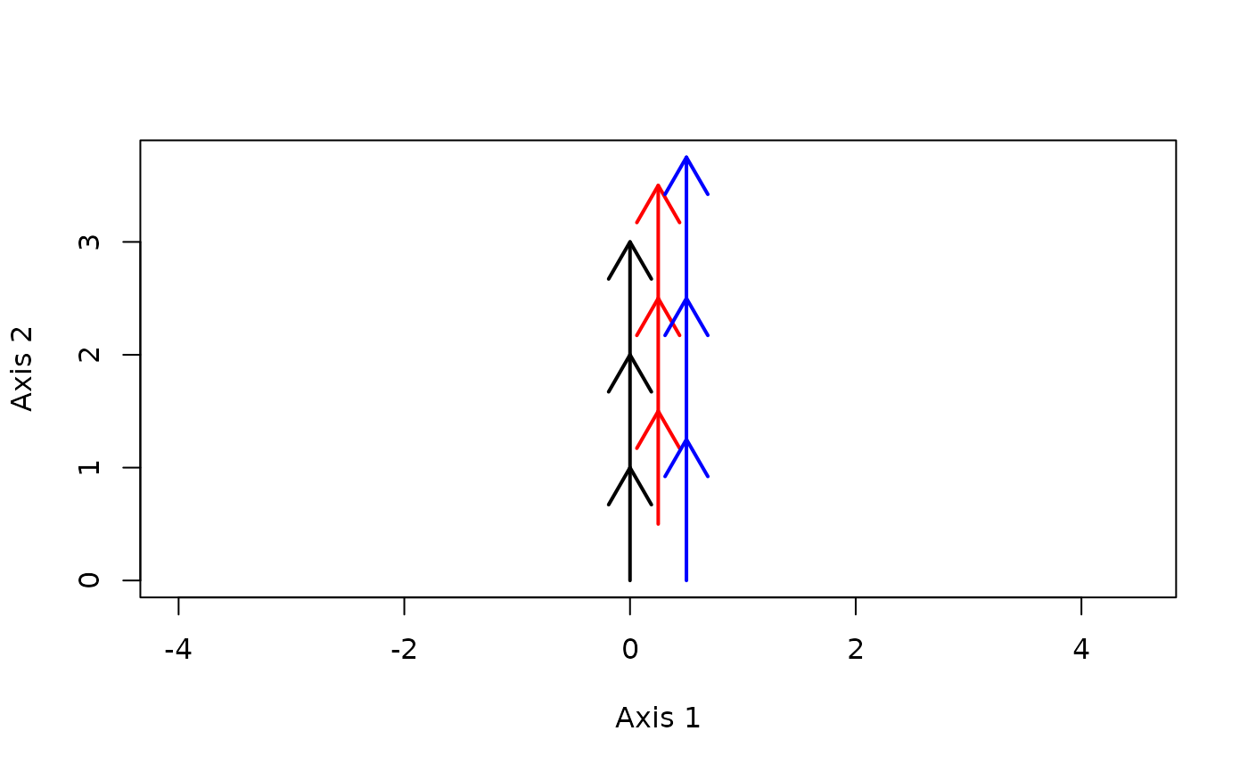
#Description of entities (sites) and surveys
entities2 <- c("1","1","1","1","2","2","2","2","3","3","3","3")
times2 <- c(1,2,3,4,1,2,3,4,1,2,3,4)
#Raw data table
xy2<-matrix(0, nrow=12, ncol=2)
xy2[2,2]<-1
xy2[3,2]<-2
xy2[4,2]<-3
xy2[5:8,1] <- 0.25
xy2[5:8,2] <- xy2[1:4,2] + 0.5 # States are all shifted with respect to site "1"
xy2[9:12,1] <- 0.5
xy2[9:12,2] <- xy2[1:4,2]*1.25 # 1.25 times faster than site "1"
#Draw trajectories
trajectoryPlot(xy2, entities2,
traj.colors = c("black","red", "blue"), lwd = 2)
#Distance matrix
d <- dist(xy)
d
#> 1 2 3 4 5 6 7
#> 2 1.0000000
#> 3 2.0000000 1.0000000
#> 4 3.0000000 2.0000000 1.0000000
#> 5 0.2500000 1.0307764 2.0155644 3.0103986
#> 6 1.0307764 0.2500000 1.0307764 2.0155644 1.0000000
#> 7 1.5811388 0.7071068 0.7071068 1.5811388 1.5206906 0.5590170
#> 8 2.2360680 1.4142136 1.0000000 1.4142136 2.1360009 1.2500000 0.7071068
#> 9 0.5000000 1.1180340 2.0615528 3.0413813 0.2500000 1.0307764 1.5000000
#> 10 1.1180340 0.5000000 1.1180340 2.0615528 1.0307764 0.2500000 0.5000000
#> 11 1.6007811 1.0307764 1.2500000 2.0155644 1.4577380 0.7905694 0.5590170
#> 12 1.8027756 1.5000000 1.8027756 2.5000000 1.6007811 1.2500000 1.1180340
#> 8 9 10 11
#> 2
#> 3
#> 4
#> 5
#> 6
#> 7
#> 8
#> 9 2.0615528
#> 10 1.1180340 1.0000000
#> 11 0.7500000 1.3462912 0.5590170
#> 12 1.1180340 1.4142136 1.0000000 0.5590170
#Trajectory data
x <- defineTrajectories(d, entities, surveys)
#Distances between trajectory segments
segmentDistances(x, distance.type = "Hausdorff")
#> $Dseg
#> 1[1-2] 1[2-3] 1[3-4] 2[1-2] 2[2-3] 2[3-4] 3[1-2]
#> 1[2-3] 1.0000000
#> 1[3-4] 2.0000000 1.0000000
#> 2[1-2] 0.2500000 1.0307764 2.0155644
#> 2[2-3] 1.0307764 0.7071068 1.5811388 1.0000000
#> 2[3-4] 1.5811388 1.0000000 1.4142136 1.5206906 0.7071068
#> 3[1-2] 0.5000000 1.1180340 2.0615528 0.2500000 1.0307764 1.5000000
#> 3[2-3] 1.1180340 1.1180340 2.0124612 1.0307764 0.5590170 0.7500000 1.0000000
#> 3[3-4] 1.6007811 1.5000000 2.0155644 1.4577380 1.1180340 1.0606602 1.3416408
#> 3[2-3]
#> 1[2-3]
#> 1[3-4]
#> 2[1-2]
#> 2[2-3]
#> 2[3-4]
#> 3[1-2]
#> 3[2-3]
#> 3[3-4] 0.5590170
#>
#> $Dini
#> 1[1-2] 1[2-3] 1[3-4] 2[1-2] 2[2-3] 2[3-4] 3[1-2]
#> 1[2-3] 1.0000000
#> 1[3-4] 2.0000000 1.0000000
#> 2[1-2] 0.2500000 1.0307764 2.0155644
#> 2[2-3] 1.0307764 0.2500000 1.0307764 1.0000000
#> 2[3-4] 1.5811388 0.7071068 0.7071068 1.5206906 0.5590170
#> 3[1-2] 0.5000000 1.1180340 2.0615528 0.2500000 1.0307764 1.5000000
#> 3[2-3] 1.1180340 0.5000000 1.1180340 1.0307764 0.2500000 0.5000000 1.0000000
#> 3[3-4] 1.6007811 1.0307764 1.2500000 1.4577380 0.7905694 0.5590170 1.3462912
#> 3[2-3]
#> 1[2-3]
#> 1[3-4]
#> 2[1-2]
#> 2[2-3]
#> 2[3-4]
#> 3[1-2]
#> 3[2-3]
#> 3[3-4] 0.5590170
#>
#> $Dfin
#> 1[1-2] 1[2-3] 1[3-4] 2[1-2] 2[2-3] 2[3-4] 3[1-2]
#> 1[2-3] 1.0000000
#> 1[3-4] 2.0000000 1.0000000
#> 2[1-2] 0.2500000 1.0307764 2.0155644
#> 2[2-3] 0.7071068 0.7071068 1.5811388 0.5590170
#> 2[3-4] 1.4142136 1.0000000 1.4142136 1.2500000 0.7071068
#> 3[1-2] 0.5000000 1.1180340 2.0615528 0.2500000 0.5000000 1.1180340
#> 3[2-3] 1.0307764 1.2500000 2.0155644 0.7905694 0.5590170 0.7500000 0.5590170
#> 3[3-4] 1.5000000 1.8027756 2.5000000 1.2500000 1.1180340 1.1180340 1.0000000
#> 3[2-3]
#> 1[2-3]
#> 1[3-4]
#> 2[1-2]
#> 2[2-3]
#> 2[3-4]
#> 3[1-2]
#> 3[2-3]
#> 3[3-4] 0.5590170
#>
#> $Dinifin
#> 1[1-2] 1[2-3] 1[3-4] 2[1-2] 2[2-3] 2[3-4] 3[1-2]
#> 1[1-2] 1.0000000 2.0000000 3.000000 1.0307764 1.5811388 2.2360680 1.118034
#> 1[2-3] 0.0000000 1.0000000 2.000000 0.2500000 0.7071068 1.4142136 0.500000
#> 1[3-4] 1.0000000 0.0000000 1.000000 1.0307764 0.7071068 1.0000000 1.118034
#> 2[1-2] 1.0307764 2.0155644 3.010399 1.0000000 1.5206906 2.1360009 1.030776
#> 2[2-3] 0.2500000 1.0307764 2.015564 0.0000000 0.5590170 1.2500000 0.250000
#> 2[3-4] 0.7071068 0.7071068 1.581139 0.5590170 0.0000000 0.7071068 0.500000
#> 3[1-2] 1.1180340 2.0615528 3.041381 1.0307764 1.5000000 2.0615528 1.000000
#> 3[2-3] 0.5000000 1.1180340 2.061553 0.2500000 0.5000000 1.1180340 0.000000
#> 3[3-4] 1.0307764 1.2500000 2.015564 0.7905694 0.5590170 0.7500000 0.559017
#> 3[2-3] 3[3-4]
#> 1[1-2] 1.6007811 1.802776
#> 1[2-3] 1.0307764 1.500000
#> 1[3-4] 1.2500000 1.802776
#> 2[1-2] 1.4577380 1.600781
#> 2[2-3] 0.7905694 1.250000
#> 2[3-4] 0.5590170 1.118034
#> 3[1-2] 1.3462912 1.414214
#> 3[2-3] 0.5590170 1.000000
#> 3[3-4] 0.0000000 0.559017
#>
segmentDistances(x, distance.type = "directed-segment")
#> $Dseg
#> 1[1-2] 1[2-3] 1[3-4] 2[1-2] 2[2-3] 2[3-4] 3[1-2]
#> 1[2-3] 1.0000000
#> 1[3-4] 2.0000000 1.0000000
#> 2[1-2] 0.2500000 1.0307764 2.0155644
#> 2[2-3] 1.0307764 0.7071068 1.5811388 1.0000000
#> 2[3-4] 1.5811388 1.0000000 1.4142136 1.5206906 0.7071068
#> 3[1-2] 0.5000000 1.1180340 2.0615528 0.2500000 1.0307764 1.5000000
#> 3[2-3] 1.1180340 1.1180340 2.0124612 1.0307764 0.5590170 0.7500000 1.0000000
#> 3[3-4] 1.6007811 1.5590170 2.0155644 1.4577380 1.1180340 1.0606602 1.5590170
#> 3[2-3]
#> 1[2-3]
#> 1[3-4]
#> 2[1-2]
#> 2[2-3]
#> 2[3-4]
#> 3[1-2]
#> 3[2-3]
#> 3[3-4] 0.5590170
#>
#> $Dini
#> 1[1-2] 1[2-3] 1[3-4] 2[1-2] 2[2-3] 2[3-4] 3[1-2]
#> 1[2-3] 1.0000000
#> 1[3-4] 2.0000000 1.0000000
#> 2[1-2] 0.2500000 1.0307764 2.0155644
#> 2[2-3] 1.0307764 0.2500000 1.0307764 1.0000000
#> 2[3-4] 1.5811388 0.7071068 0.7071068 1.5206906 0.5590170
#> 3[1-2] 0.5000000 1.1180340 2.0615528 0.2500000 1.0307764 1.5000000
#> 3[2-3] 1.1180340 0.5000000 1.1180340 1.0307764 0.2500000 0.5000000 1.0000000
#> 3[3-4] 1.6007811 1.0307764 1.2500000 1.4577380 0.7905694 0.5590170 1.3462912
#> 3[2-3]
#> 1[2-3]
#> 1[3-4]
#> 2[1-2]
#> 2[2-3]
#> 2[3-4]
#> 3[1-2]
#> 3[2-3]
#> 3[3-4] 0.5590170
#>
#> $Dfin
#> 1[1-2] 1[2-3] 1[3-4] 2[1-2] 2[2-3] 2[3-4] 3[1-2]
#> 1[2-3] 1.0000000
#> 1[3-4] 2.0000000 1.0000000
#> 2[1-2] 0.2500000 1.0307764 2.0155644
#> 2[2-3] 0.7071068 0.7071068 1.5811388 0.5590170
#> 2[3-4] 1.4142136 1.0000000 1.4142136 1.2500000 0.7071068
#> 3[1-2] 0.5000000 1.1180340 2.0615528 0.2500000 0.5000000 1.1180340
#> 3[2-3] 1.0307764 1.2500000 2.0155644 0.7905694 0.5590170 0.7500000 0.5590170
#> 3[3-4] 1.5000000 1.8027756 2.5000000 1.2500000 1.1180340 1.1180340 1.0000000
#> 3[2-3]
#> 1[2-3]
#> 1[3-4]
#> 2[1-2]
#> 2[2-3]
#> 2[3-4]
#> 3[1-2]
#> 3[2-3]
#> 3[3-4] 0.5590170
#>
#> $Dinifin
#> 1[1-2] 1[2-3] 1[3-4] 2[1-2] 2[2-3] 2[3-4] 3[1-2]
#> 1[1-2] 1.0000000 2.0000000 3.000000 1.0307764 1.5811388 2.2360680 1.118034
#> 1[2-3] 0.0000000 1.0000000 2.000000 0.2500000 0.7071068 1.4142136 0.500000
#> 1[3-4] 1.0000000 0.0000000 1.000000 1.0307764 0.7071068 1.0000000 1.118034
#> 2[1-2] 1.0307764 2.0155644 3.010399 1.0000000 1.5206906 2.1360009 1.030776
#> 2[2-3] 0.2500000 1.0307764 2.015564 0.0000000 0.5590170 1.2500000 0.250000
#> 2[3-4] 0.7071068 0.7071068 1.581139 0.5590170 0.0000000 0.7071068 0.500000
#> 3[1-2] 1.1180340 2.0615528 3.041381 1.0307764 1.5000000 2.0615528 1.000000
#> 3[2-3] 0.5000000 1.1180340 2.061553 0.2500000 0.5000000 1.1180340 0.000000
#> 3[3-4] 1.0307764 1.2500000 2.015564 0.7905694 0.5590170 0.7500000 0.559017
#> 3[2-3] 3[3-4]
#> 1[1-2] 1.6007811 1.802776
#> 1[2-3] 1.0307764 1.500000
#> 1[3-4] 1.2500000 1.802776
#> 2[1-2] 1.4577380 1.600781
#> 2[2-3] 0.7905694 1.250000
#> 2[3-4] 0.5590170 1.118034
#> 3[1-2] 1.3462912 1.414214
#> 3[2-3] 0.5590170 1.000000
#> 3[3-4] 0.0000000 0.559017
#>
#Distances between trajectories
trajectoryDistances(x, distance.type = "Hausdorff")
#> 1 2
#> 2 2.015564
#> 3 2.061553 1.500000
trajectoryDistances(x, distance.type = "DSPD")
#> 1 2
#> 2 0.7214045
#> 3 1.1345910 0.5714490
#Trajectory convergence/divergence
trajectoryConvergence(x)
#> $tau
#> 1 2 3
#> 1 NA 0.9128709 0.9128709
#> 2 0.9128709 NA 0.9128709
#> 3 0.9128709 0.6666667 NA
#>
#> $p.value
#> 1 2 3
#> 1 NA 0.07095149 0.07095149
#> 2 0.07095149 NA 0.07095149
#> 3 0.07095149 0.33333333 NA
#>
#Trajectory dynamic correspondence
trajectoryCorrespondence(x)
#> 1 2 3
#> 1 NA 4.363029 2.242967
#> 2 0.052 NA 2.775852
#> 3 0.082 0.083000 NA
#### Example of trajectory shifts
#Description of entities (sites) and surveys
entities2 <- c("1","1","1","1","2","2","2","2","3","3","3","3")
times2 <- c(1,2,3,4,1,2,3,4,1,2,3,4)
#Raw data table
xy2<-matrix(0, nrow=12, ncol=2)
xy2[2,2]<-1
xy2[3,2]<-2
xy2[4,2]<-3
xy2[5:8,1] <- 0.25
xy2[5:8,2] <- xy2[1:4,2] + 0.5 # States are all shifted with respect to site "1"
xy2[9:12,1] <- 0.5
xy2[9:12,2] <- xy2[1:4,2]*1.25 # 1.25 times faster than site "1"
#Draw trajectories
trajectoryPlot(xy2, entities2,
traj.colors = c("black","red", "blue"), lwd = 2)
 #Trajectory data
x2 <- defineTrajectories(dist(xy2), entities2, times = times2)
#Check that the third trajectory is faster
trajectorySpeeds(x2)
#> S1 S2 S3 Path
#> 1 1.00 1.00 1.00 1.00
#> 2 1.00 1.00 1.00 1.00
#> 3 1.25 1.25 1.25 1.25
#Trajectory shifts
trajectoryShifts(x2)
#> reference site survey time timeRef shift
#> 1 1 2 1 1 1.50 0.50
#> 2 1 2 2 2 2.50 0.50
#> 3 1 2 3 3 3.50 0.50
#> 4 1 2 4 4 NA NA
#> 5 1 3 1 1 1.00 0.00
#> 6 1 3 2 2 2.25 0.25
#> 7 1 3 3 3 3.50 0.50
#> 8 1 3 4 4 NA NA
#> 9 2 1 1 1 NA NA
#> 10 2 1 2 2 1.50 -0.50
#> 11 2 1 3 3 2.50 -0.50
#> 12 2 1 4 4 3.50 -0.50
#> 13 2 3 1 1 NA NA
#> 14 2 3 2 2 1.75 -0.25
#> 15 2 3 3 3 3.00 0.00
#> 16 2 3 4 4 NA NA
#> 17 3 1 1 1 1.00 0.00
#> 18 3 1 2 2 1.80 -0.20
#> 19 3 1 3 3 2.60 -0.40
#> 20 3 1 4 4 3.40 -0.60
#> 21 3 2 1 1 1.40 0.40
#> 22 3 2 2 2 2.20 0.20
#> 23 3 2 3 3 3.00 0.00
#> 24 3 2 4 4 3.80 -0.20
#Trajectory data
x2 <- defineTrajectories(dist(xy2), entities2, times = times2)
#Check that the third trajectory is faster
trajectorySpeeds(x2)
#> S1 S2 S3 Path
#> 1 1.00 1.00 1.00 1.00
#> 2 1.00 1.00 1.00 1.00
#> 3 1.25 1.25 1.25 1.25
#Trajectory shifts
trajectoryShifts(x2)
#> reference site survey time timeRef shift
#> 1 1 2 1 1 1.50 0.50
#> 2 1 2 2 2 2.50 0.50
#> 3 1 2 3 3 3.50 0.50
#> 4 1 2 4 4 NA NA
#> 5 1 3 1 1 1.00 0.00
#> 6 1 3 2 2 2.25 0.25
#> 7 1 3 3 3 3.50 0.50
#> 8 1 3 4 4 NA NA
#> 9 2 1 1 1 NA NA
#> 10 2 1 2 2 1.50 -0.50
#> 11 2 1 3 3 2.50 -0.50
#> 12 2 1 4 4 3.50 -0.50
#> 13 2 3 1 1 NA NA
#> 14 2 3 2 2 1.75 -0.25
#> 15 2 3 3 3 3.00 0.00
#> 16 2 3 4 4 NA NA
#> 17 3 1 1 1 1.00 0.00
#> 18 3 1 2 2 1.80 -0.20
#> 19 3 1 3 3 2.60 -0.40
#> 20 3 1 4 4 3.40 -0.60
#> 21 3 2 1 1 1.40 0.40
#> 22 3 2 2 2 2.20 0.20
#> 23 3 2 3 3 3.00 0.00
#> 24 3 2 4 4 3.80 -0.20