Draws cummulative abundance profiles

Create plots used to inspect one or more cumulative abundance profiles.

# S3 method for CAP
plot(x, sizes=NULL, species=NULL, plots=NULL, switchAxes=FALSE, 
                   add=FALSE, drawAxes = TRUE, xlab="", ylab="", type="s",...)
# S3 method for stratifiedvegdata
plot(x, sizes=NULL, species=NULL, plots=NULL, switchAxes=FALSE, 
                   add=FALSE, drawAxes = TRUE, xlab="", ylab="", type="s",...)

Arguments

x

An object returned from function CAP or an object of class stratifiedvegdata (see documentation for function stratifyvegdata).

sizes

A vector containing the size values associated to each size class. If NULL the y-axis will be defined using the size class order in x.

species

A vector of strings indicating the species whose profile is to be drawn. If NULL all species are plotted.

plots

A vector indicating the plot records whose profile is to be drawn. Can be a character vector (for plot names), a numeric vector (for plot indices) or a logical vector (for TRUE/FALSE selection). If NULL all plot records are plotted.

switchAxes

A flag indicating whether ordinate and abscissa axes should be interchanged.

add

A flag indicating whether profiles should be drawn on top of current drawing area. If add=FALSE a new plot is created.

drawAxes

A flag indicating whether axes should be drawn.

xlab

String label for the x axis.

ylab

String label for the y axis.

type

Type of plot to be drawn ("p" for points, "l" for lines, "s" for steps, ...).

...

Additional plotting parameters.

References

De Cáceres, M., Legendre, P. & He, F. (2013) Dissimilarity measurements and the size structure of ecological communities. Methods in Ecology and Evolution 4: 1167-1177.

Author

Miquel De Cáceres, CREAF

See also

CAP

Examples

## Load stratified data
data(medreg)

## Check that 'medreg' has correct class
class(medreg)
#> [1] "stratifiedvegdata" "list"             

## Create cumulative abundance profile (CAP) for each plot
medreg.CAP = CAP(medreg)

## Draw the stratified data and profile corresponding to the third plot
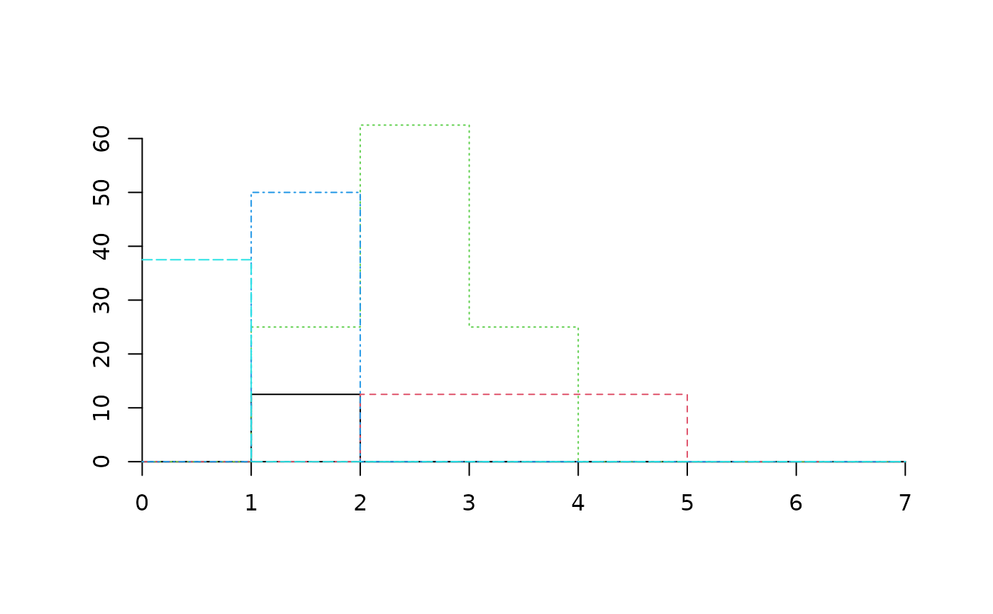
plot(medreg, plots="3")

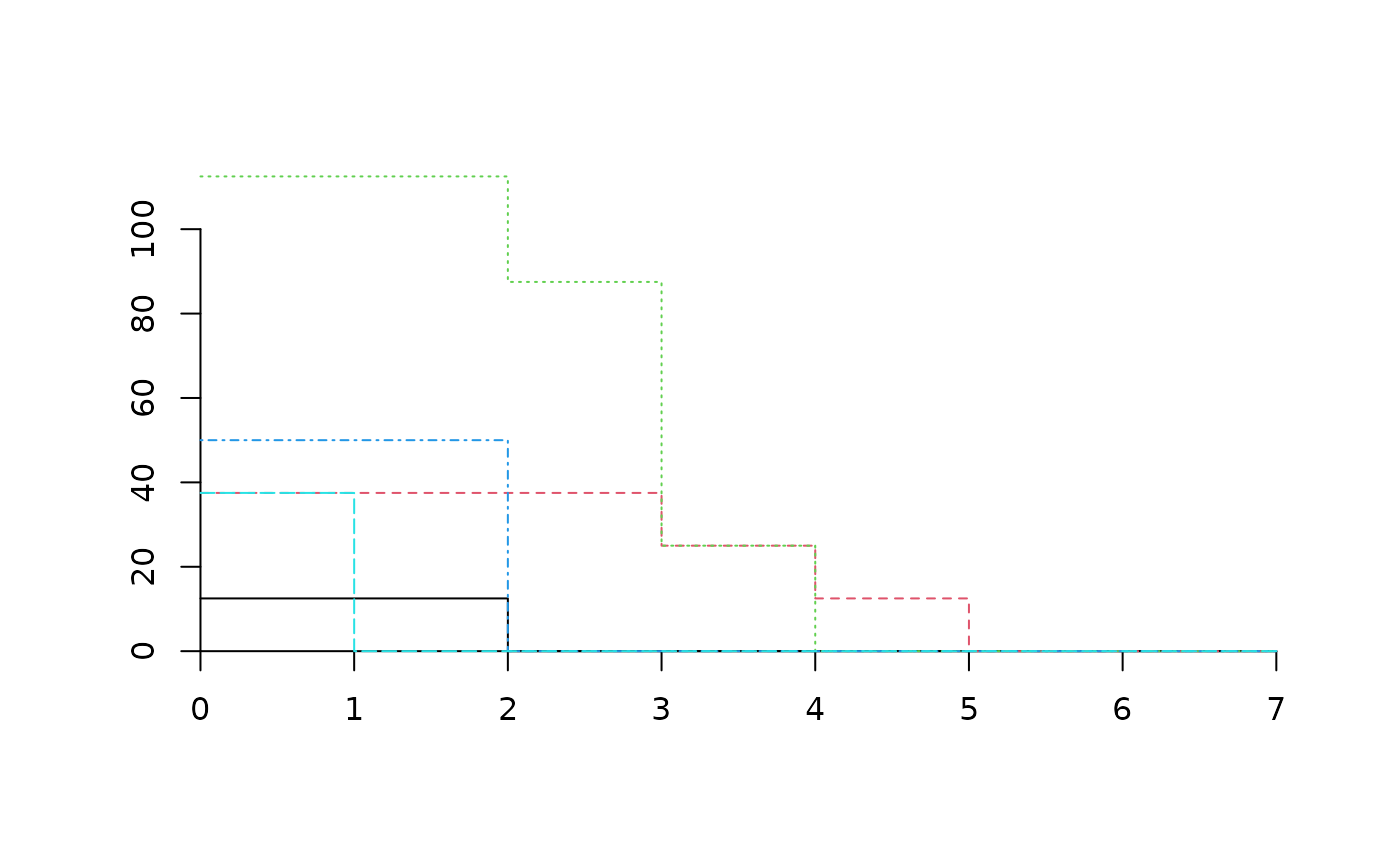
plot(medreg.CAP, plots="3")


## Look at the plot and CAP of the same plot
medreg[["3"]]
#>                                1    2    3    4    5 6 7
#> Pine trees                   0.0 12.5  0.0  0.0  0.0 0 0
#> Quercus trees                0.0  0.0 12.5 12.5 12.5 0 0
#> Tall shrubs and small trees  0.0 25.0 62.5 25.0  0.0 0 0
#> Scrubs and small shrubs      0.0 50.0  0.0  0.0  0.0 0 0
#> Grass                       37.5  0.0  0.0  0.0  0.0 0 0
medreg.CAP[["3"]]
#>                                 1     2    3  4    5 6 7
#> Pine trees                   12.5  12.5  0.0  0  0.0 0 0
#> Quercus trees                37.5  37.5 37.5 25 12.5 0 0
#> Tall shrubs and small trees 112.5 112.5 87.5 25  0.0 0 0
#> Scrubs and small shrubs      50.0  50.0  0.0  0  0.0 0 0
#> Grass                        37.5   0.0  0.0  0  0.0 0 0