Draws a cummulative abundance surface

Create plots used to inspect one or more cumulative abundance profiles.

# S3 method for CAS
plot(x, plot=NULL, species=NULL, sizes1=NULL, sizes2 = NULL, 
                   palette = colorRampPalette(c( "light blue","light green","white", 
                   "yellow","orange","red")), zlim=NULL,...)

Arguments

x

An object of class CAS.

plot

A string indicating the plot record whose surface is to be drawn.

species

A string indicating the species whose profile is to be drawn.

sizes1

A vector containing the size values associated to each primary size class. If NULL the x-axis will be defined using the primary size class order in x.

sizes2

A vector containing the size values associated to each secondary size class. If NULL the y-axis will be defined using the secondary size class order in x.

palette

Color palette for z values.

zlim

The limits for the z-axis.

...

Additional plotting parameters for function persp.

References

De Cáceres, M., Legendre, P. & He, F. (2013) Dissimilarity measurements and the size structure of ecological communities. Methods in Ecology and Evolution 4: 1167-1177.

Author

Miquel De Cáceres, CREAF

See also

CAS, persp

Examples

## Create synthetic tree data
pl = rep(1,100) # All trees in the same plot
sp = ifelse(runif(100)>0.5,1,2) # Random species identity (species 1 or 2)
h=rgamma(100,10,2) # Heights (m)
d = rpois(100, lambda=h^2) # Diameters (cm)
m = data.frame(plot=pl,species=sp, height=h,diameter=d) 
m$ba = pi*(m$diameter/200)^2
print(head(m))
#>   plot species   height diameter         ba
#> 1    1       1 5.031797       21 0.03463606
#> 2    1       1 4.562974       18 0.02544690
#> 3    1       2 7.091567       49 0.18857410
#> 4    1       1 5.523011       32 0.08042477
#> 5    1       2 3.604555       12 0.01130973
#> 6    1       2 4.069347       15 0.01767146

## Size classes
heights = seq(0,4, by=.25)^2 # Quadratic classes
diams = seq(0,130, by=5) # Linear classes

## Stratify tree data
X<-stratifyvegdata(m, sizes1=heights, sizes2=diams, 
                   plotColumn = "plot", speciesColumn = "species", 
                   size1Column = "height", size2Column = "diameter", 
                   abundanceColumn = "ba")


## Build cummulative abundance surface
Y = CAS(X)

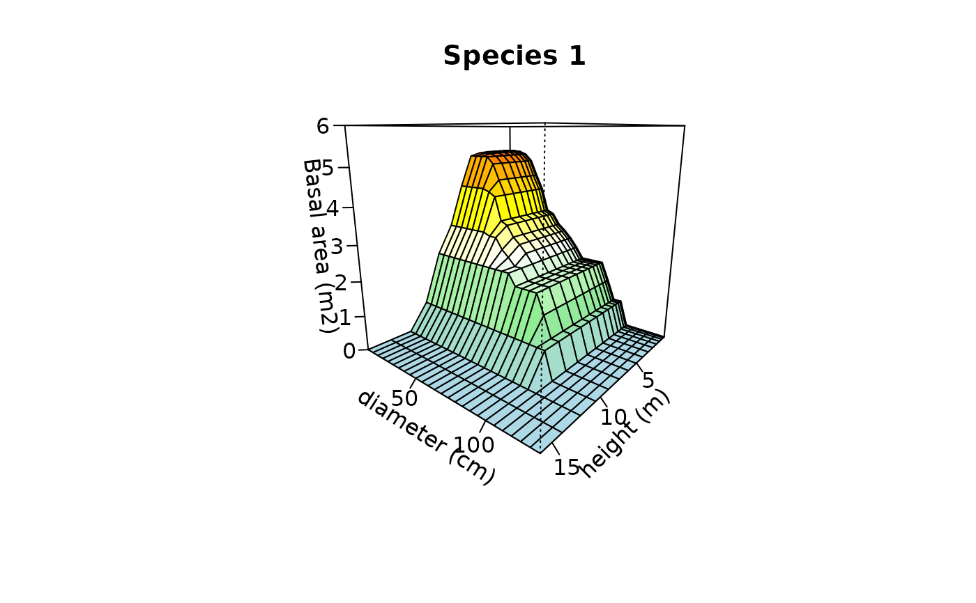
## Plot the surface of species '1' in plot '1' using heights and diameters
plot(Y, species=1, sizes1=heights[-1], xlab="height (m)", 
     ylab="diameter (cm)", sizes2=diams[-1], zlab="Basal area (m2)",
     zlim = c(0,6), main="Species 1")