Forest dynamics
Miquel De Caceres
2026-07-04
Source:vignettes/runmodels/ForestDynamics.Rmd
ForestDynamics.RmdAbout this vignette
This document describes how to run the forest dynamics model of
medfate, described in De Cáceres et al. (2023) and
implemented in function fordyn(). This document is meant to
teach users to run the simulation model with function
fordyn(). Details of the model design and formulation can
be found at the corresponding chapters of the medfate
book.
Because the model builds on the growth and water balance models, the
reader is assumed here to be familiarized with spwb() and
growth() (otherwise read vignettes Basic
water balance and Forest
growth).
Preparing model inputs
Any forest dynamics model needs information on climate, vegetation
and soils of the forest stand to be simulated. Moreover, since models in
medfate differentiate between species, information on
species-specific model parameters is also needed. In this subsection we
explain the different steps to prepare the data needed to run function
fordyn().
Model inputs are explained in greater detail in vignettes Understanding
model inputs and Preparing
model inputs. Here we only review the different steps required
to run function fordyn().
Soil, vegetation, meteorology and species data
Soil information needs to be entered as a data frame
with soil layers in rows and physical attributes in columns. Soil
physical attributes can be initialized to default values, for a given
number of layers, using function defaultSoilParams():
examplesoil <- defaultSoilParams(4)
examplesoil
## widths clay sand om nitrogen ph bd rfc
## 1 300 25 25 NA NA NA 1.5 25
## 2 700 25 25 NA NA NA 1.5 45
## 3 1000 25 25 NA NA NA 1.5 75
## 4 2000 25 25 NA NA NA 1.5 95As explained in the package overview, models included in
medfate were primarily designed to be ran on forest
inventory plots. Here we use the example object provided with
the package:
data(exampleforest)
exampleforest
## $treeData
## Species DBH Height N Z50 Z95
## 1 Pinus halepensis 37.55 800 168 100 300
## 2 Quercus ilex 14.60 660 384 300 1000
##
## $shrubData
## Species Height Cover Z50 Z95
## 1 Quercus coccifera 80 3.75 200 1000
##
## attr(,"class")
## [1] "forest" "list"We can keep track of cohort age if we define a column called
Age in tree or shrub data, for example let us assume we
know the age of the two tree cohorts:
exampleforest$treeData$Age <- c(40, 24)Importantly, a data frame with daily weather for the period to be simulated is required. Here we use the default data frame included with the package:
##        dates MinTemperature MaxTemperature Precipitation MinRelativeHumidity
## 1 2001-01-01     -0.5934215       6.287950      4.869109            65.15411
## 2 2001-01-02     -2.3662458       4.569737      2.498292            57.43761
## 3 2001-01-03     -3.8541036       2.661951      0.000000            58.77432
## 4 2001-01-04     -1.8744860       3.097705      5.796973            66.84256
## 5 2001-01-05      0.3288287       7.551532      1.884401            62.97656
## 6 2001-01-06      0.5461322       7.186784     13.359801            74.25754
##   MaxRelativeHumidity Radiation WindSpeed
## 1           100.00000  12.89251  2.000000
## 2            94.71780  13.03079  7.662544
## 3            94.66823  16.90722  2.000000
## 4            95.80950  11.07275  2.000000
## 5           100.00000  13.45205  7.581347
## 6           100.00000  12.84841  6.570501
Finally, simulations in medfate require a data frame
with species parameter values, which we load using defaults for
Catalonia (NE Spain):
data("SpParamsMED")Simulation control
Apart from data inputs, the behaviour of simulation models can be
controlled using a set of global parameters. The default
parameterization is obtained using function
defaultControl():
control <- defaultControl("Granier")Here we will run simulations of forest dynamics using the basic water
balance model (i.e. transpirationMode = "Granier"). The
complexity of the soil water balance calculations can be changed by
using "Sperry" as input to defaultControl().
However, when running fordyn() sub-daily output will never
be stored (i.e. setting subdailyResults = TRUE is
useless).
Executing the forest dynamics model
In this vignette we will fake a ten-year weather input by repeating the example weather data frame ten times.
meteo <- rbind(examplemeteo, examplemeteo, examplemeteo, examplemeteo,
                    examplemeteo, examplemeteo, examplemeteo, examplemeteo,
                    examplemeteo, examplemeteo)
meteo$dates <- as.character(seq(as.Date("2001-01-01"),
                                as.Date("2010-12-29"), by="day"))
Now we run the forest dynamics model using all inputs (note that no
intermediate input object is needed, as in spwb() or
growth()):
fd<-fordyn(exampleforest, examplesoil, SpParamsMED, meteo, control,
           latitude = 41.82592, elevation = 100)
## Simulating year 2001 (1/10): (a) Growth/mortality, (b) Regeneration nT = 2 nS = 1
## Simulating year 2002 (2/10): (a) Growth/mortality, (b) Regeneration nT = 2 nS = 1
## Simulating year 2003 (3/10): (a) Growth/mortality, (b) Regeneration nT = 2 nS = 1
## Simulating year 2004 (4/10): (a) Growth/mortality, (b) Regeneration nT = 2 nS = 1
## Simulating year 2005 (5/10): (a) Growth/mortality, (b) Regeneration nT = 2 nS = 1
## Simulating year 2006 (6/10): (a) Growth/mortality, (b) Regeneration nT = 2 nS = 1
## Simulating year 2007 (7/10): (a) Growth/mortality, (b) Regeneration nT = 2 nS = 1
## Simulating year 2008 (8/10): (a) Growth/mortality, (b) Regeneration nT = 2 nS = 1
## Simulating year 2009 (9/10): (a) Growth/mortality, (b) Regeneration nT = 2 nS = 1
## Simulating year 2010 (10/10): (a) Growth/mortality, (b) Regeneration nT = 2 nS = 1It is worth noting that, while fordyn() calls function
growth() internally for each simulated year, the
verbose option of the control parameters only affects
function fordyn() (i.e. all console output from
growth() is hidden). Recruitment and summaries are done
only once a year at the level of function fordyn().
Inspecting model outputs
Stand, species and cohort summaries and plots
Among other outputs, function fordyn() calculates
standard summary statistics that describe the structural and
compositional state of the forest at each time step. For example, we can
access stand-level statistics using:
fd$StandSummary## Step NumTreeSpecies NumTreeCohorts NumShrubSpecies NumShrubCohorts
## 1 0 2 2 1 1
## 2 1 2 2 1 1
## 3 2 2 2 1 1
## 4 3 2 2 1 1
## 5 4 2 2 1 1
## 6 5 2 2 1 1
## 7 6 2 2 1 1
## 8 7 2 2 1 1
## 9 8 2 2 1 1
## 10 9 2 2 1 1
## 11 10 2 2 1 1
## TreeDensityLive TreeBasalAreaLive DominantTreeHeight DominantTreeDiameter
## 1 552.0000 25.03330 800 37.55
## 2 551.3698 24.99465 800 37.55
## 3 550.7418 24.95615 800 37.55
## 4 550.1161 24.91781 800 37.55
## 5 549.4908 24.87952 800 37.55
## 6 548.8695 24.84148 800 37.55
## 7 548.2504 24.80361 800 37.55
## 8 547.6335 24.76588 800 37.55
## 9 547.0170 24.72820 800 37.55
## 10 546.4044 24.69078 800 37.55
## 11 545.7973 24.65371 800 37.55
## QuadraticMeanTreeDiameter HartBeckingIndex ShrubCoverLive BasalAreaDead
## 1 24.02949 53.20353 3.750000 0.00000000
## 2 24.02465 53.23393 3.843800 0.03865577
## 3 24.01982 53.26427 3.944028 0.03849813
## 4 24.01501 53.29456 4.045493 0.03834160
## 5 24.01020 53.32487 4.149415 0.03829058
## 6 24.00542 53.35504 4.254012 0.03803142
## 7 24.00065 53.38516 4.360165 0.03787816
## 8 23.99589 53.41522 4.468359 0.03772598
## 9 23.99114 53.44531 4.579249 0.03767760
## 10 23.98641 53.47526 4.690252 0.03742437
## 11 23.98173 53.50500 4.805726 0.03707150
## ShrubCoverDead BasalAreaCut ShrubCoverCut
## 1 0.000000000 0 0
## 2 0.005823228 0 0
## 3 0.005971755 0 0
## 4 0.006126578 0 0
## 5 0.006301411 0 0
## 6 0.006444460 0 0
## 7 0.006606231 0 0
## 8 0.006770733 0 0
## 9 0.006957953 0 0
## 10 0.007109529 0 0
## 11 0.007242598 0 0Species-level analogous statistics are shown using:
fd$SpeciesSummary## Step Species NumCohorts TreeDensityLive TreeBasalAreaLive
## 1 0 Pinus halepensis 1 168.0000 18.604547
## 2 0 Quercus coccifera 1 NA NA
## 3 0 Quercus ilex 1 384.0000 6.428755
## 4 1 Pinus halepensis 1 167.7010 18.571436
## 5 1 Quercus coccifera 1 NA NA
## 6 1 Quercus ilex 1 383.6688 6.423209
## 7 2 Pinus halepensis 1 167.4033 18.538467
## 8 2 Quercus coccifera 1 NA NA
## 9 2 Quercus ilex 1 383.3385 6.417680
## 10 3 Pinus halepensis 1 167.1069 18.505638
## 11 3 Quercus coccifera 1 NA NA
## 12 3 Quercus ilex 1 383.0092 6.412168
## 13 4 Pinus halepensis 1 166.8109 18.472860
## 14 4 Quercus coccifera 1 NA NA
## 15 4 Quercus ilex 1 382.6800 6.406656
## 16 5 Pinus halepensis 1 166.5169 18.440309
## 17 5 Quercus coccifera 1 NA NA
## 18 5 Quercus ilex 1 382.3526 6.401175
## 19 6 Pinus halepensis 1 166.2242 18.407896
## 20 6 Quercus coccifera 1 NA NA
## 21 6 Quercus ilex 1 382.0262 6.395710
## 22 7 Pinus halepensis 1 165.9328 18.375618
## 23 7 Quercus coccifera 1 NA NA
## 24 7 Quercus ilex 1 381.7007 6.390262
## 25 8 Pinus halepensis 1 165.6417 18.343389
## 26 8 Quercus coccifera 1 NA NA
## 27 8 Quercus ilex 1 381.3753 6.384814
## 28 9 Pinus halepensis 1 165.3527 18.311382
## 29 9 Quercus coccifera 1 NA NA
## 30 9 Quercus ilex 1 381.0517 6.379396
## 31 10 Pinus halepensis 1 165.0665 18.279683
## 32 10 Quercus coccifera 1 NA NA
## 33 10 Quercus ilex 1 380.7308 6.374024
## ShrubCoverLive BasalAreaDead ShrubCoverDead BasalAreaCut ShrubCoverCut
## 1 NA 0.000000000 NA 0 NA
## 2 3.750000 NA 0.000000000 NA 0
## 3 NA 0.000000000 NA 0 NA
## 4 NA 0.033110412 NA 0 NA
## 5 3.843800 NA 0.005823228 NA 0
## 6 NA 0.005545358 NA 0 NA
## 7 NA 0.032969074 NA 0 NA
## 8 3.944028 NA 0.005971755 NA 0
## 9 NA 0.005529053 NA 0 NA
## 10 NA 0.032828755 NA 0 NA
## 11 4.045493 NA 0.006126578 NA 0
## 12 NA 0.005512844 NA 0 NA
## 13 NA 0.032778812 NA 0 NA
## 14 4.149415 NA 0.006301411 NA 0
## 15 NA 0.005511767 NA 0 NA
## 16 NA 0.032550751 NA 0 NA
## 17 4.254012 NA 0.006444460 NA 0
## 18 NA 0.005480665 NA 0 NA
## 19 NA 0.032413426 NA 0 NA
## 20 4.360165 NA 0.006606231 NA 0
## 21 NA 0.005464738 NA 0 NA
## 22 NA 0.032277079 NA 0 NA
## 23 4.468359 NA 0.006770733 NA 0
## 24 NA 0.005448903 NA 0 NA
## 25 NA 0.032229573 NA 0 NA
## 26 4.579249 NA 0.006957953 NA 0
## 27 NA 0.005448024 NA 0 NA
## 28 NA 0.032006910 NA 0 NA
## 29 4.690252 NA 0.007109529 NA 0
## 30 NA 0.005417464 NA 0 NA
## 31 NA 0.031699151 NA 0 NA
## 32 4.805726 NA 0.007242598 NA 0
## 33 NA 0.005372345 NA 0 NAPackage medfate provides a simple plot
function for objects of class fordyn. For example, we can
show the interannual variation in stand-level basal area using:
plot(fd, type = "StandBasalArea")
Tree/shrub tables
Another useful output of fordyn() are tables in long
format with cohort structural information (i.e. DBH, height, density,
etc) for each time step:
fd$TreeTable## Step Year Cohort Species DBH Height N Z50 Z95 Z100 Age
## 1 0 NA T1_148 Pinus halepensis 37.55 800 168.0000 100 300 NA 40
## 2 0 NA T2_168 Quercus ilex 14.60 660 384.0000 300 1000 NA 24
## 3 1 2001 T1_148 Pinus halepensis 37.55 800 167.7010 100 300 NA 40
## 4 1 2001 T2_168 Quercus ilex 14.60 660 383.6688 300 1000 NA 24
## 5 2 2002 T1_148 Pinus halepensis 37.55 800 167.4033 100 300 NA 41
## 6 2 2002 T2_168 Quercus ilex 14.60 660 383.3385 300 1000 NA 25
## 7 3 2003 T1_148 Pinus halepensis 37.55 800 167.1069 100 300 NA 42
## 8 3 2003 T2_168 Quercus ilex 14.60 660 383.0092 300 1000 NA 26
## 9 4 2004 T1_148 Pinus halepensis 37.55 800 166.8109 100 300 NA 43
## 10 4 2004 T2_168 Quercus ilex 14.60 660 382.6800 300 1000 NA 27
## 11 5 2005 T1_148 Pinus halepensis 37.55 800 166.5169 100 300 NA 44
## 12 5 2005 T2_168 Quercus ilex 14.60 660 382.3526 300 1000 NA 28
## 13 6 2006 T1_148 Pinus halepensis 37.55 800 166.2242 100 300 NA 45
## 14 6 2006 T2_168 Quercus ilex 14.60 660 382.0262 300 1000 NA 29
## 15 7 2007 T1_148 Pinus halepensis 37.55 800 165.9328 100 300 NA 46
## 16 7 2007 T2_168 Quercus ilex 14.60 660 381.7007 300 1000 NA 30
## 17 8 2008 T1_148 Pinus halepensis 37.55 800 165.6417 100 300 NA 47
## 18 8 2008 T2_168 Quercus ilex 14.60 660 381.3753 300 1000 NA 31
## 19 9 2009 T1_148 Pinus halepensis 37.55 800 165.3527 100 300 NA 48
## 20 9 2009 T2_168 Quercus ilex 14.60 660 381.0517 300 1000 NA 32
## 21 10 2010 T1_148 Pinus halepensis 37.55 800 165.0665 100 300 NA 49
## 22 10 2010 T2_168 Quercus ilex 14.60 660 380.7308 300 1000 NA 33
## ObsID
## 1 <NA>
## 2 <NA>
## 3 NA
## 4 NA
## 5 NA
## 6 NA
## 7 NA
## 8 NA
## 9 NA
## 10 NA
## 11 NA
## 12 NA
## 13 NA
## 14 NA
## 15 NA
## 16 NA
## 17 NA
## 18 NA
## 19 NA
## 20 NA
## 21 NA
## 22 NAThe same can be shown for dead trees:
fd$DeadTreeTable## Step Year Cohort Species DBH Height N N_starvation
## 1 1 2001 T1_148 Pinus halepensis 37.55 800 0.2989887 0
## 2 1 2001 T2_168 Quercus ilex 14.60 660 0.3312333 0
## 3 2 2002 T1_148 Pinus halepensis 37.55 800 0.2977124 0
## 4 2 2002 T2_168 Quercus ilex 14.60 660 0.3302594 0
## 5 3 2003 T1_148 Pinus halepensis 37.55 800 0.2964453 0
## 6 3 2003 T2_168 Quercus ilex 14.60 660 0.3292911 0
## 7 4 2004 T1_148 Pinus halepensis 37.55 800 0.2959943 0
## 8 4 2004 T2_168 Quercus ilex 14.60 660 0.3292268 0
## 9 5 2005 T1_148 Pinus halepensis 37.55 800 0.2939349 0
## 10 5 2005 T2_168 Quercus ilex 14.60 660 0.3273691 0
## 11 6 2006 T1_148 Pinus halepensis 37.55 800 0.2926949 0
## 12 6 2006 T2_168 Quercus ilex 14.60 660 0.3264177 0
## 13 7 2007 T1_148 Pinus halepensis 37.55 800 0.2914637 0
## 14 7 2007 T2_168 Quercus ilex 14.60 660 0.3254719 0
## 15 8 2008 T1_148 Pinus halepensis 37.55 800 0.2910347 0
## 16 8 2008 T2_168 Quercus ilex 14.60 660 0.3254193 0
## 17 9 2009 T1_148 Pinus halepensis 37.55 800 0.2890240 0
## 18 9 2009 T2_168 Quercus ilex 14.60 660 0.3235940 0
## 19 10 2010 T1_148 Pinus halepensis 37.55 800 0.2862449 0
## 20 10 2010 T2_168 Quercus ilex 14.60 660 0.3208989 0
## N_dessication N_burnt N_resprouting_stumps Z50 Z95 Z100 Age ObsID
## 1 0 0 0 100 300 NA 40 NA
## 2 0 0 0 300 1000 NA 24 NA
## 3 0 0 0 100 300 NA 40 NA
## 4 0 0 0 300 1000 NA 24 NA
## 5 0 0 0 100 300 NA 41 NA
## 6 0 0 0 300 1000 NA 25 NA
## 7 0 0 0 100 300 NA 42 NA
## 8 0 0 0 300 1000 NA 26 NA
## 9 0 0 0 100 300 NA 43 NA
## 10 0 0 0 300 1000 NA 27 NA
## 11 0 0 0 100 300 NA 44 NA
## 12 0 0 0 300 1000 NA 28 NA
## 13 0 0 0 100 300 NA 45 NA
## 14 0 0 0 300 1000 NA 29 NA
## 15 0 0 0 100 300 NA 46 NA
## 16 0 0 0 300 1000 NA 30 NA
## 17 0 0 0 100 300 NA 47 NA
## 18 0 0 0 300 1000 NA 31 NA
## 19 0 0 0 100 300 NA 48 NA
## 20 0 0 0 300 1000 NA 32 NAAccessing the output from function growth()
Since function fordyn() makes internal calls to function
growth(), it stores the result in a vector called
GrowthResults, which we can use to inspect intra-annual
patterns of desired variables. For example, the following shows the leaf
area for individuals of the three cohorts during the second year:
plot(fd$GrowthResults[[2]], "LeafArea", bySpecies = T)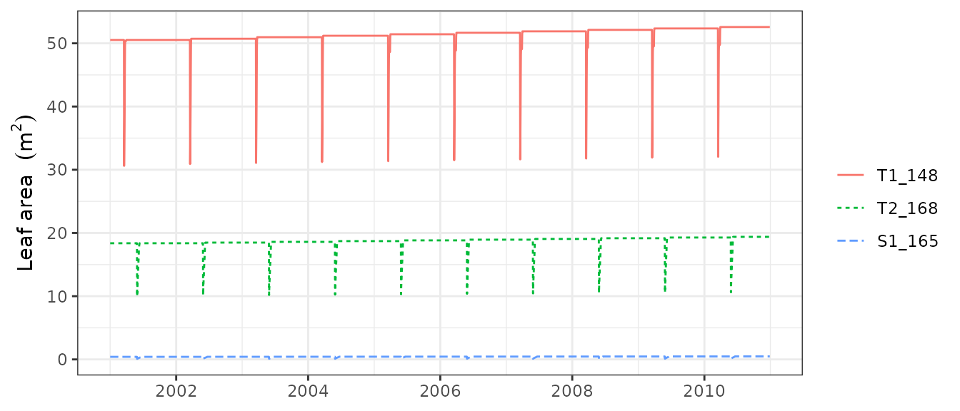 Instead of examining year by year, it is possible to plot the whole
series of results by passing a
Instead of examining year by year, it is possible to plot the whole
series of results by passing a fordyn object to the
plot() function:
plot(fd, "LeafArea")
We can also create interactive plots for particular steps using
function shinyplot(), e.g.:
shinyplot(fd$GrowthResults[[1]])Finally, calling function extract() will extract and
bind outputs for all the internal calls to function
growth():
## # A tibble: 3,650 × 53
##    date           PET Precipitation    Rain   Snow NetRain Snowmelt Infiltration
##    <date>     [L/m^2]       [L/m^2] [L/m^2] [L/m^… [L/m^2]  [L/m^2]      [L/m^2]
##  1 2001-01-01   0.883          4.87    4.87   0      3.30      0           3.30
##  2 2001-01-02   1.64           2.50    2.50   0      0.972     0           0.972
##  3 2001-01-03   1.30           0       0      0      0         0           0
##  4 2001-01-04   0.569          5.80    5.80   0      4.24      0           4.24
##  5 2001-01-05   1.68           1.88    1.88   0      0.733     0           0.733
##  6 2001-01-06   1.21          13.4    13.4    0     11.6       0          11.6
##  7 2001-01-07   0.637          5.38    0      5.38   0         0           0
##  8 2001-01-08   0.832          0       0      0      0         0           0
##  9 2001-01-09   1.98           0       0      0      0         0           0
## 10 2001-01-10   0.829          5.12    5.12   0      3.55      5.38        8.92
## # ℹ 3,640 more rows
## # ℹ 45 more variables: InfiltrationExcess [L/m^2], SaturationExcess [L/m^2],
## #   Runoff [L/m^2], DeepDrainage [L/m^2], CapillarityRise [L/m^2],
## #   Evapotranspiration [L/m^2], Interception [L/m^2], SoilEvaporation [L/m^2],
## #   HerbTranspiration [L/m^2], PlantExtraction [L/m^2], Transpiration [L/m^2],
## #   MistletoeTranspiration [L/m^2], HydraulicRedistribution [L/m^2],
## #   LAI [m^2/m^2], LAIherb [m^2/m^2], LAIlive [m^2/m^2], …
Forest dynamics including management
The package allows including forest management in simulations of
forest dynamics. This is done in a very flexible manner, in the sense
that fordyn() allows the user to supply an arbitrary
function implementing a desired management strategy for the stand whose
dynamics are to be simulated. The package includes, however, an in-built
default function called defaultManagementFunction() along
with a flexible parameterization, a list with defaults provided by
function defaultManagementArguments().
Here we provide an example of simulations including forest management:
# Default arguments
args <- defaultManagementArguments()
# Here one can modify defaults before calling fordyn()
#
# Simulation
fd<-fordyn(exampleforest, examplesoil, SpParamsMED, meteo, control,
           latitude = 41.82592, elevation = 100,
           management_function = defaultManagementFunction,
           management_args = args)
## Simulating year 2001 (1/10): (a) Growth/mortality & management [thinning], (b) Regeneration nT = 2 nS = 2
## Simulating year 2002 (2/10): (a) Growth/mortality & management [none], (b) Regeneration nT = 2 nS = 2
## Simulating year 2003 (3/10): (a) Growth/mortality & management [none], (b) Regeneration nT = 2 nS = 2
## Simulating year 2004 (4/10): (a) Growth/mortality & management [none], (b) Regeneration nT = 2 nS = 2
## Simulating year 2005 (5/10): (a) Growth/mortality & management [none], (b) Regeneration nT = 2 nS = 2
## Simulating year 2006 (6/10): (a) Growth/mortality & management [none], (b) Regeneration nT = 2 nS = 2
## Simulating year 2007 (7/10): (a) Growth/mortality & management [none], (b) Regeneration nT = 2 nS = 2
## Simulating year 2008 (8/10): (a) Growth/mortality & management [none], (b) Regeneration nT = 2 nS = 2
## Simulating year 2009 (9/10): (a) Growth/mortality & management [none], (b) Regeneration nT = 2 nS = 2
## Simulating year 2010 (10/10): (a) Growth/mortality & management [none], (b) Regeneration nT = 2 nS = 2When management is included in simulations, two additional tables are produced, corresponding to the trees and shrubs that were cut, e.g.:
fd$CutTreeTable## Step Year Cohort Species DBH Height N Z50 Z95 Z100 Age
## 1 1 2001 T1_148 Pinus halepensis 37.55 800 9.708976 100 300 NA 40
## 2 1 2001 T2_168 Quercus ilex 14.60 660 383.668767 300 1000 NA 24
## ObsID
## 1 NA
## 2 NAManagement parameters were those of an irregular model with thinning interventions from ‘below’, indicating that smaller trees were to be cut earlier:
args$type## [1] "irregular"
args$thinning## [1] "below"Note that in this example, there is resprouting of Quercus ilex after the thinning intervention, evidenced by the new cohort (T3_168) appearing in year 2001:
fd$TreeTable## Step Year Cohort Species DBH Height N Z50 Z95 Z100
## 1 0 NA T1_148 Pinus halepensis 37.55 800.00000 168.0000 100 300 NA
## 2 0 NA T2_168 Quercus ilex 14.60 660.00000 384.0000 300 1000 NA
## 3 1 2001 T1_148 Pinus halepensis 37.55 800.00000 157.9920 100 300 NA
## 4 1 2001 T3_168 Quercus ilex 1.00 47.23629 3000.0000 300 1000 NA
## 5 2 2002 T1_148 Pinus halepensis 37.55 800.00000 157.8237 100 300 NA
## 6 2 2002 T3_168 Quercus ilex 1.00 47.23629 2998.3124 300 1000 NA
## 7 3 2003 T1_148 Pinus halepensis 37.55 800.00000 157.6559 100 300 NA
## 8 3 2003 T3_168 Quercus ilex 1.00 47.23629 2996.6277 300 1000 NA
## 9 4 2004 T1_148 Pinus halepensis 37.55 800.00000 157.4880 100 300 NA
## 10 4 2004 T3_168 Quercus ilex 1.00 47.23629 2994.9414 300 1000 NA
## 11 5 2005 T1_148 Pinus halepensis 37.55 800.00000 157.3209 100 300 NA
## 12 5 2005 T3_168 Quercus ilex 1.00 47.23629 2993.2627 300 1000 NA
## 13 6 2006 T1_148 Pinus halepensis 37.55 800.00000 157.1543 100 300 NA
## 14 6 2006 T3_168 Quercus ilex 1.00 47.23629 2991.5870 300 1000 NA
## 15 7 2007 T1_148 Pinus halepensis 37.55 800.00000 156.9881 100 300 NA
## 16 7 2007 T3_168 Quercus ilex 1.00 47.23629 2989.9141 300 1000 NA
## 17 8 2008 T1_148 Pinus halepensis 37.55 800.00000 156.8219 100 300 NA
## 18 8 2008 T3_168 Quercus ilex 1.00 47.23629 2988.2397 300 1000 NA
## 19 9 2009 T1_148 Pinus halepensis 37.55 800.00000 156.6565 100 300 NA
## 20 9 2009 T3_168 Quercus ilex 1.00 47.23629 2986.5727 300 1000 NA
## 21 10 2010 T1_148 Pinus halepensis 37.55 800.00000 156.4925 100 300 NA
## 22 10 2010 T3_168 Quercus ilex 1.00 47.23629 2984.9177 300 1000 NA
## Age ObsID
## 1 40 <NA>
## 2 24 <NA>
## 3 40 NA
## 4 24 <NA>
## 5 41 NA
## 6 24 NA
## 7 42 NA
## 8 25 NA
## 9 43 NA
## 10 26 NA
## 11 44 NA
## 12 27 NA
## 13 45 NA
## 14 28 NA
## 15 46 NA
## 16 29 NA
## 17 47 NA
## 18 30 NA
## 19 48 NA
## 20 31 NA
## 21 49 NA
## 22 32 NAReferences
- De Cáceres M, Molowny-Horas R, Cabon A, Martínez-Vilalta J, Mencuccini M, García-Valdés R, Nadal-Sala D, Sabaté S, Martin-StPaul N, Morin X, D’Adamo F, Batllori E, Améztegui A (2023) MEDFATE 2.9.3: A trait-enabled model to simulate Mediterranean forest function and dynamics at regional scales. Geoscientific Model Development 16: 3165-3201 (https://doi.org/10.5194/gmd-16-3165-2023).