Basic water balance

About this vignette

The present document describes how to run the soil plant water balance model described in De Cáceres et al. (2015) using package medfate. The document illustrates how to prepare the inputs, use the simulation functions and inspect the outputs. All the details of the model design and formulation can be found at the medfatebook. Because it introduces many basic features of simulations with package medfate, this document should be read before addressing advanced topics of water balance simulations or growth simulations.

Preparing model inputs

Model inputs are explained in greater detail in vignettes Understanding model inputs and Preparing model inputs. Here we only review the different steps required to run function spwb().

Soil, vegetation, meteorology and species data

Soil information needs to be entered as a data frame with soil layers in rows and physical attributes in columns. Soil physical attributes can be initialized to default values, for a given number of layers, using function defaultSoilParams():

spar <- defaultSoilParams(4)

The soil input for water balance simulation is actually a list of class soil that is created using a function with the same name:

examplesoil <- soil(spar)

As explained in the package overview, models included in medfate were primarily designed to be ran on forest inventory plots. Here we use the example object provided with the package:

data(exampleforest)
exampleforest

## $treeData
##            Species   N   DBH Height Z50  Z95
## 1 Pinus halepensis 168 37.55    800 100  600
## 2     Quercus ilex 384 14.60    660 300 1000
## 
## $shrubData
##             Species Cover Height Z50  Z95
## 1 Quercus coccifera  3.75     80 200 1000
## 
## $herbCover
## [1] 10
## 
## $herbHeight
## [1] 20
## 
## $seedBank
## [1] Species Percent
## <0 rows> (or 0-length row.names)
## 
## attr(,"class")
## [1] "forest" "list"

Importantly, a data frame with daily weather for the period to be simulated is required. Here we use the default data frame included with the package:

data(examplemeteo)
head(examplemeteo)

##        dates MinTemperature MaxTemperature Precipitation MinRelativeHumidity
## 1 2001-01-01     -0.5934215       6.287950      4.869109            65.15411
## 2 2001-01-02     -2.3662458       4.569737      2.498292            57.43761
## 3 2001-01-03     -3.8541036       2.661951      0.000000            58.77432
## 4 2001-01-04     -1.8744860       3.097705      5.796973            66.84256
## 5 2001-01-05      0.3288287       7.551532      1.884401            62.97656
## 6 2001-01-06      0.5461322       7.186784     13.359801            74.25754
##   MaxRelativeHumidity Radiation WindSpeed
## 1           100.00000  12.89251  2.000000
## 2            94.71780  13.03079  7.662544
## 3            94.66823  16.90722  2.000000
## 4            95.80950  11.07275  2.000000
## 5           100.00000  13.45205  7.581347
## 6           100.00000  12.84841  6.570501

Finally, simulations in medfate require a data frame with species parameter values, which we load using defaults for Catalonia (NE Spain):

data("SpParamsMED")

Simulation control

Apart from data inputs, the behaviour of simulation models can be controlled using a set of global parameters. The default parameterization is obtained using function defaultControl():

control <- defaultControl("Granier")

Some parameters deserve explanation here:

Console output can be turned off by setting verbose = FALSE.
The soil water retention curves can be switched between Saxton’s and Van Genuchten’s using parameter soilFunctions.
The complexity of the soil water balance calculations will be very different if we set transpirationMode = "Sperry" or transpirationMode = "Sureau", instead of transpirationMode = "Granier".

Water balance input object

A last object is needed before calling simulation functions, called spwbInput. It consists in the compilation of aboveground and belowground parameters and the specification of additional parameter values for each plant cohort. This is done by calling function spwbInput(), but if one has a forest object, the object can be generated more directly using function forest2spwbInput():

x <- forest2spwbInput(exampleforest, examplesoil, SpParamsMED, control)

Different parameter variables will be drawn depending on the value of transpirationMode. For the basic water balance model (transpirationMode = "Granier"), relatively few parameters are needed. All the input information for forest data and species parameter values can be inspected by accessing the different elements of this object, whose names are.

names(x)

##  [1] "control"             "soil"                "canopy"             
##  [4] "herbLAI"             "herbLAImax"          "cohorts"            
##  [7] "above"               "below"               "belowLayers"        
## [10] "paramsPhenology"     "paramsAnatomy"       "paramsInterception" 
## [13] "paramsTranspiration" "paramsWaterStorage"  "internalPhenology"  
## [16] "internalWater"       "internalFCCS"

Finally, note that users can set cohort-specific parameters for soil water balance (instead of using species-level values) by modifying manually the parameter values in this object. Since some parameters may be coordinated by design, however, it is better to use specific package functions for this purpose.

Executing the soil water balance model

Water balance for a single day

Soil water balance simulations will normally span periods of several months or years, but since the model operates at a daily temporal scale, it is possible to perform soil water balance for one day only. This is done using function spwb_day(). In the following code we select day 100 from the meteorological input data and perform soil water balance for that day only:

d <- 100
date <- examplemeteo$dates[d]
meteovec <- unlist(examplemeteo[d,])
sd1<-spwb_day(x, date, meteovec,  
             latitude = 41.82592, elevation = 100, slope= 0, aspect = 0)

## Package 'meteoland' [ver. 2.2.1]

Function spwb_day() is most useful when working with the complex transpiration model. This is why so many meteorological variables are required. The output of spwb_day() is a list with five elements:

names(sd1)

## [1] "cohorts"      "topography"   "weather"      "WaterBalance" "Soil"        
## [6] "Stand"        "Plants"

cohorts: Table with the species code and species name of each cohort.
WaterBalance: Contains the soil water balance flows (precipitation, infiltration, transpiration, …)
Soil: Contains output values by soil layer (i.e. water evaporated from each soil layer, water transpired from each soil layer and the final soil water potential).
Stand: A list with stand LAI (expanded and dead leaves), canopy water retention capacity and the proportion of light (SWR or PAR) reaching the ground.
Plants: Contains output values by plant cohort (i.e. LAI values, transpiration, water potential, drought stress index, …).

sd1

## $cohorts
##         SP              Name
## T1_148 148  Pinus halepensis
## T2_168 168      Quercus ilex
## S1_165 165 Quercus coccifera
## 
## $topography
## elevation     slope    aspect 
##       100         0         0 
## 
## $weather
##        tday        prec        tmin        tmax       rhmin       rhmax 
##   6.2323731   0.0000000   0.3881289  10.0320962  42.0207334  82.3036989 
##         rad        wind        Catm        Patm         pet        rint 
##  28.7201692   3.3228840 386.0000000          NA   3.9023342   1.5000000 
## 
## $WaterBalance
##                     PET                    Rain                    Snow 
##            3.9023342059            0.0000000000            0.0000000000 
##                 NetRain                Snowmelt                   Runon 
##            0.0000000000            0.0000000000            0.0000000000 
##            Infiltration      InfiltrationExcess        SaturationExcess 
##            0.0000000000            0.0000000000            0.0000000000 
##                  Runoff            DeepDrainage         CapillarityRise 
##            0.0000000000            0.0058794508            0.0000268069 
##         SoilEvaporation       HerbTranspiration         PlantExtraction 
##            0.5000000000            0.0487254203            0.6686838719 
##           Transpiration HydraulicRedistribution 
##            0.6686838719            0.0000000000 
## 
## $Soil
##   HerbTranspiration HydraulicInput HydraulicOutput PlantExtraction         psi
## 1       0.008571001              0      0.48671421      0.48671421 -0.03555958
## 2       0.012000080              0      0.16122392      0.16122392 -0.03321178
## 3       0.013576976              0      0.01660923      0.01660923 -0.03299066
## 4       0.014577363              0      0.00413651      0.00413651 -0.03297531
## 
## $Stand
##         LAI     LAIherb     LAIlive LAIexpanded     LAIdead          Cm 
##   1.7585845   0.1736369   1.5849476   1.5849476   0.0000000   1.3904846 
##  LgroundPAR  LgroundSWR 
##  40.0075402  50.7329667 
## 
## $Plants
##               LAI    LAIlive     FPAR AbsorbedSWRFraction Extraction
## T1_148 0.84874773 0.84874773 92.18285           35.076344 0.40874422
## T2_168 0.70557382 0.70557382 72.36365           30.444383 0.23318589
## S1_165 0.03062604 0.03062604 44.32407            2.366131 0.02675376
##        Transpiration GrossPhotosynthesis PlantPsi         DDS   StemRWC
## T1_148    0.40874422           2.7741548   -0.033 0.005808769 0.9998350
## T2_168    0.23318589           2.1058696   -0.033 0.010612890 0.9997489
## S1_165    0.02675376           0.1635903   -0.033 0.003088161 0.9983684
##          LeafRWC      LFMC StemPLC     LeafPLC WaterBalance
## T1_148 0.9979679 125.89003       0 0.003069557            0
## T2_168 0.9986794  93.07448       0 0.000000000            0
## S1_165 0.9987207  96.39176       0 0.000000000            0
## 
## attr(,"class")
## [1] "spwb_day" "list"

Water balance for multiple days

Most often, users will use function spwb() to run the soil water balance model. This function requires the spwbInput object and the meteorological data frame. However, function spwb_day() by default modifies the state variables of the input objects. In particular, the values of soil moisture are now:

x$soil$W

## [1] 0.9842305 0.9986498 1.0000597 1.0001580

We simply reset state variables to their default values so that new simulations are not affected by the end state of the previous simulation:

resetInputs(x)
x$soil$W

## [1] 1 1 1 1

Now we are ready to call function spwb():

S <- spwb(x, examplemeteo, latitude = 41.82592, elevation = 100)

## Initial plant water content (mm): 7.05859
## Initial soil water content (mm): 290.875
## Initial snowpack content (mm): 0
## Performing daily simulations
## 
##  [Year 2001]:....................................
## 
## Final plant water content (mm): 7.0593
## Final soil water content (mm): 350.868
## Final snowpack content (mm): 0
## Change in plant water content (mm): 0.000700883
## Plant water balance result (mm): 0.000700883
## Change in soil water content (mm): 59.9933
## Soil water balance result (mm): 59.9933
## Change in snowpack water content (mm): 0
## Snowpack water balance result (mm): -7.10543e-15
## Water balance components:
##   Precipitation (mm) 513 Rain (mm) 462 Snow (mm) 51
##   Interception (mm) 92 Net rainfall (mm) 370
##   Infiltration (mm) 390 Infiltration excess (mm) 31 Saturation excess (mm) 0 Capillarity rise (mm) 2
##   Soil evaporation (mm) 10  Herbaceous transpiration (mm) 14 Woody plant transpiration (mm) 187
##   Plant extraction from soil (mm) 187  Plant water balance (mm) 0 Hydraulic redistribution (mm) 2
##   Runoff (mm) 31 Deep drainage (mm) 122

Function spwb() returns an object of class with the same name, actually a list:

class(S)

## [1] "spwb" "list"

If we inspect its elements, we realize that the output is arranged differently than in spwb_day():

names(S)

## [1] "latitude"     "topography"   "weather"      "spwbInput"    "spwbOutput"  
## [6] "WaterBalance" "Soil"         "Stand"        "Plants"

In particular, element spwbInput contains a copy of the input parameters that were used to run the model:

names(S$spwbInput)

##  [1] "control"             "soil"                "canopy"             
##  [4] "herbLAI"             "herbLAImax"          "cohorts"            
##  [7] "above"               "below"               "belowLayers"        
## [10] "paramsPhenology"     "paramsAnatomy"       "paramsInterception" 
## [13] "paramsTranspiration" "paramsWaterStorage"  "internalPhenology"  
## [16] "internalWater"       "internalFCCS"

As before, WaterBalance contains water balance components, but in this case in form of a data frame with days in rows:

head(S$WaterBalance)

##                  PET Precipitation      Rain Snow    NetRain Snowmelt
## 2001-01-01 0.8828475      4.869109  4.869109    0  3.4241795        0
## 2001-01-02 1.6375337      2.498292  2.498292    0  1.0717469        0
## 2001-01-03 1.3017026      0.000000  0.000000    0  0.0000000        0
## 2001-01-04 0.5690790      5.796973  5.796973    0  4.3625616        0
## 2001-01-05 1.6760567      1.884401  1.884401    0  0.7539027        0
## 2001-01-06 1.2077028     13.359801 13.359801    0 11.7240275        0
##            Infiltration InfiltrationExcess SaturationExcess Runoff DeepDrainage
## 2001-01-01    3.4241795                  0                0      0  0.005453485
## 2001-01-02    1.0717469                  0                0      0  0.005216676
## 2001-01-03    0.0000000                  0                0      0  0.005017641
## 2001-01-04    4.3625616                  0                0      0  0.005200701
## 2001-01-05    0.7539027                  0                0      0  0.005869696
## 2001-01-06   11.7240275                  0                0      0  0.005890970
##            CapillarityRise Evapotranspiration Interception SoilEvaporation
## 2001-01-01    4.316996e-05          2.0551277     1.444929      0.44789475
## 2001-01-02    1.894436e-05          1.7950032     1.426545      0.06716959
## 2001-01-03    0.000000e+00          0.2959936     0.000000      0.05645746
## 2001-01-04    3.170545e-04          1.6060978     1.434411      0.06697917
## 2001-01-05    0.000000e+00          1.4656495     1.130499      0.02644820
## 2001-01-06    4.331022e-03          1.8842477     1.635773      0.02602566
##            HerbTranspiration PlantExtraction Transpiration
## 2001-01-01       0.011023432      0.15128020    0.15128020
## 2001-01-02       0.020448154      0.28084078    0.28084078
## 2001-01-03       0.016254782      0.22328135    0.22328135
## 2001-01-04       0.007106185      0.09760108    0.09760108
## 2001-01-05       0.020931015      0.28777147    0.28777147
## 2001-01-06       0.015082123      0.20736677    0.20736677
##            HydraulicRedistribution
## 2001-01-01             0.000000000
## 2001-01-02             0.017679718
## 2001-01-03             0.014393466
## 2001-01-04             0.006500031
## 2001-01-05             0.019396272
## 2001-01-06             0.014283588

Element Plants is in turn a list with several dataframes with plant output variables, for example plant water potentials are in:

head(S$Plants$PlantPsi)

##                 T1_148      T2_168      S1_165
## 2001-01-01 -0.03300000 -0.03300000 -0.03300000
## 2001-01-02 -0.02947344 -0.03049298 -0.03000187
## 2001-01-03 -0.02881534 -0.02997653 -0.02941892
## 2001-01-04 -0.02941957 -0.03033070 -0.02989424
## 2001-01-05 -0.02469534 -0.02699417 -0.02590380
## 2001-01-06 -0.02454389 -0.02678800 -0.02572610

Inspecting model outputs

Plots

Package medfate provides a simple plot function for objects of class spwb. It can be used to show meteorological inputs, snow dynamics, and different components of the water balance:

plot(S, type = "PET_Precipitation")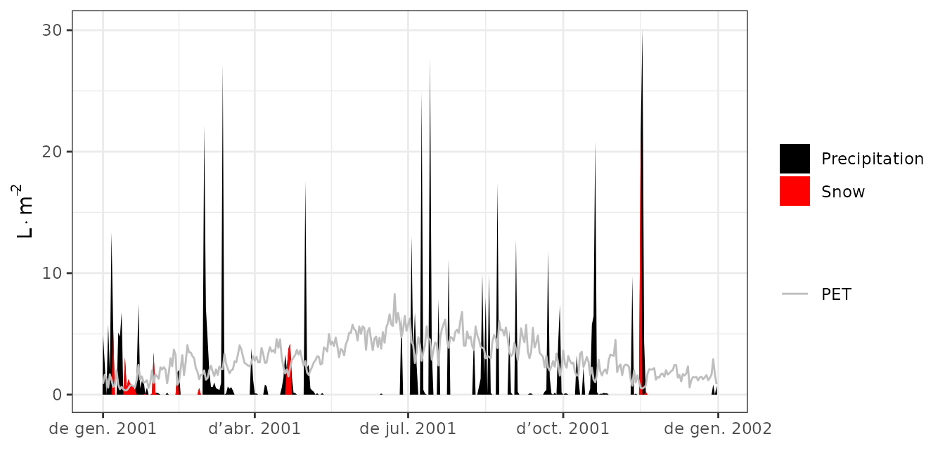

plot(S, type = "Snow")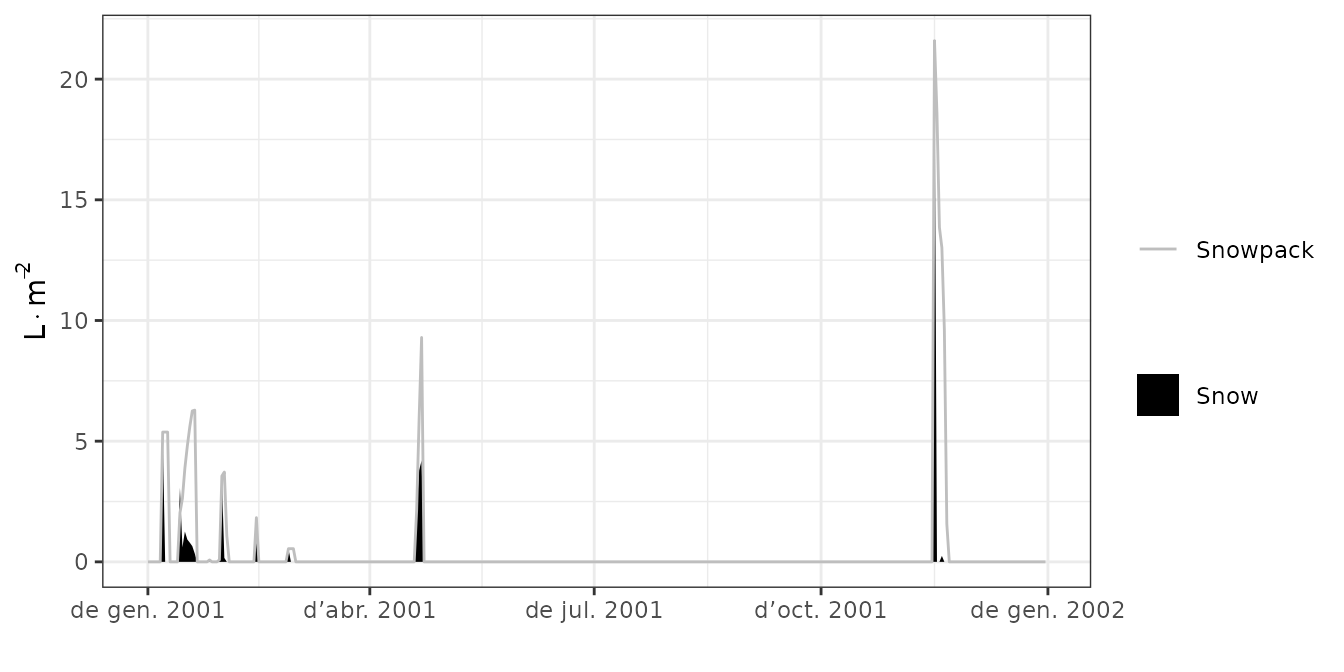

plot(S, type = "Export")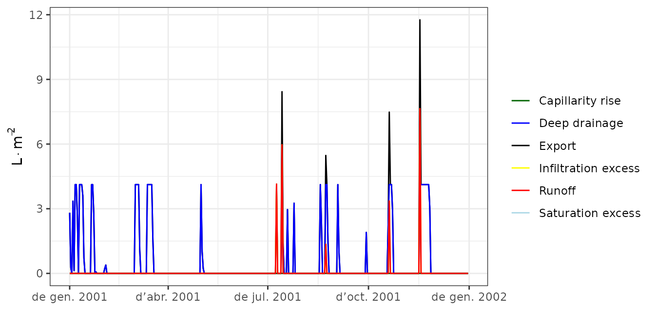

plot(S, type = "Evapotranspiration")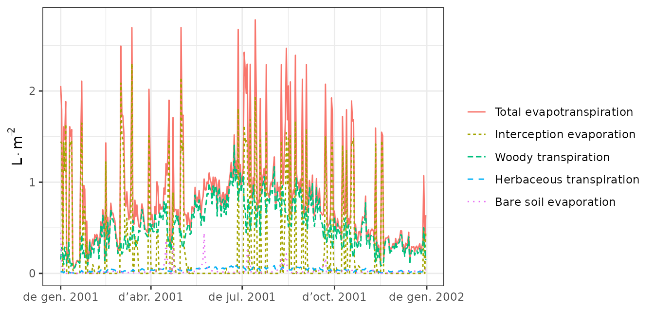

Function plot is also allows displaying soil moisture dynamics by layer, which can be done in four different ways (the first two only imply a change in axis units):

plot(S, type="SoilTheta")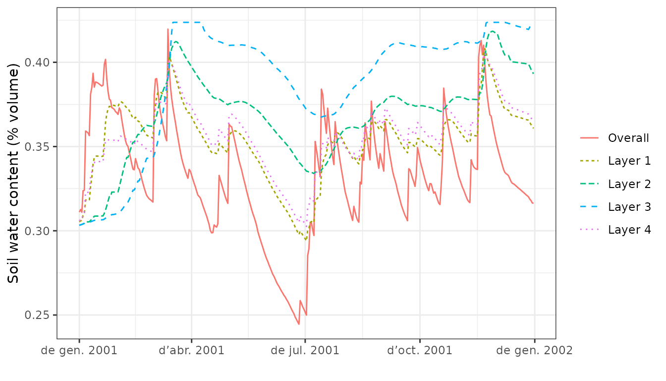

plot(S, type="SoilRWC")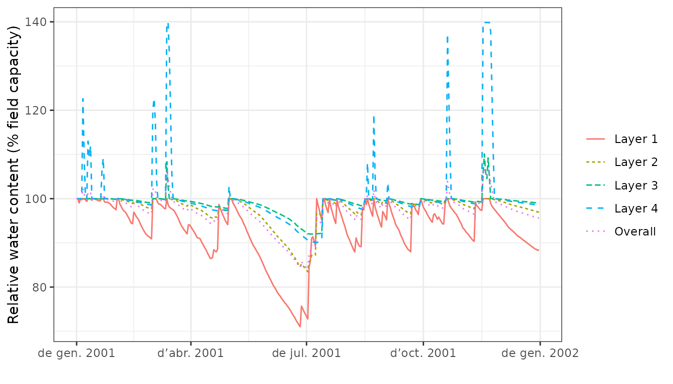

plot(S, type="SoilPsi")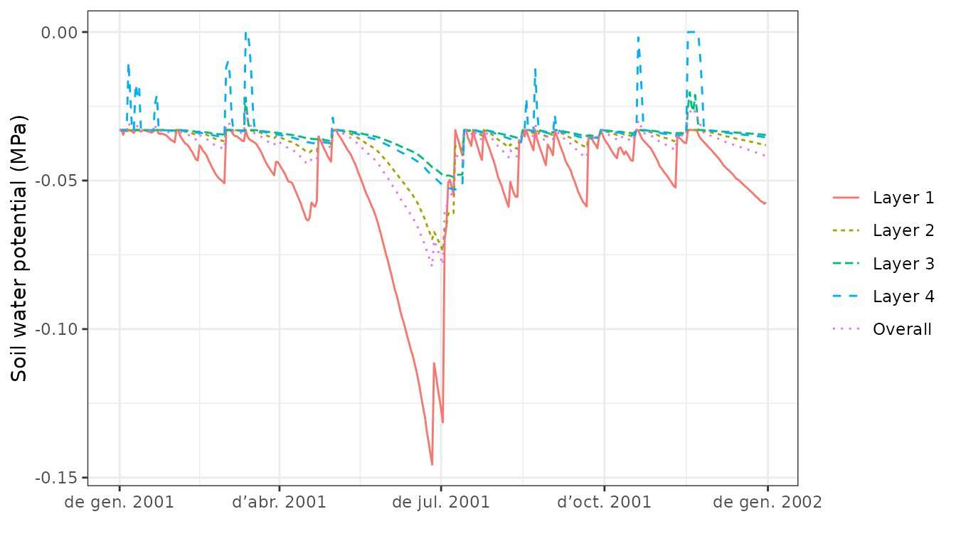

plot(S, type="SoilVol")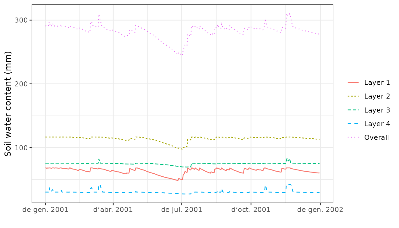

Finally, the same function can also be used to draw the dynamics of plant variables by cohorts, such as transpiration, gross photosynthesis or water potential:

plot(S, type="Transpiration")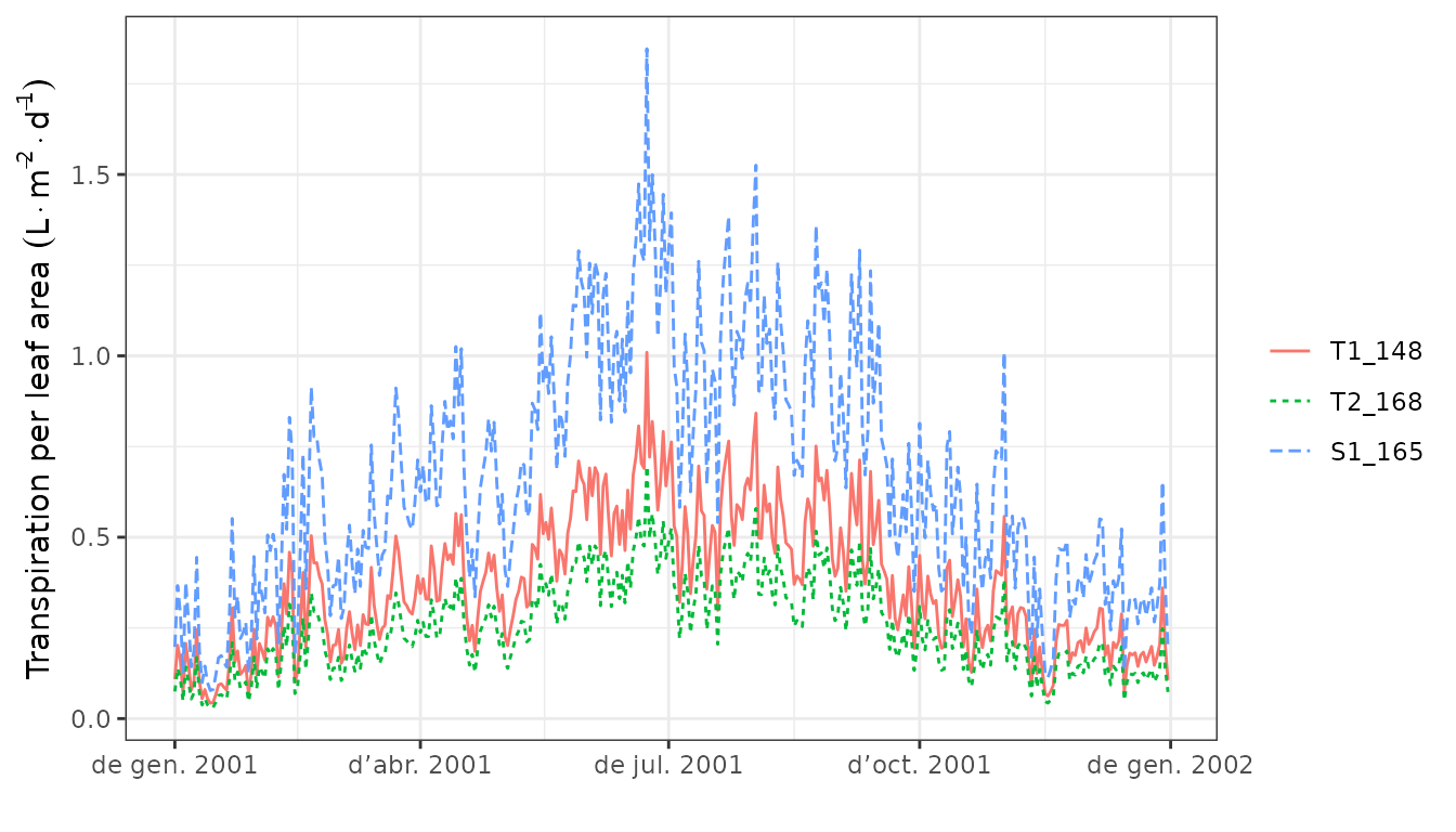

plot(S, type="GrossPhotosynthesis")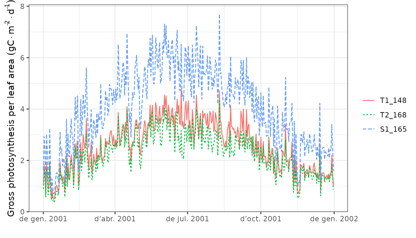

plot(S, type="PlantPsi")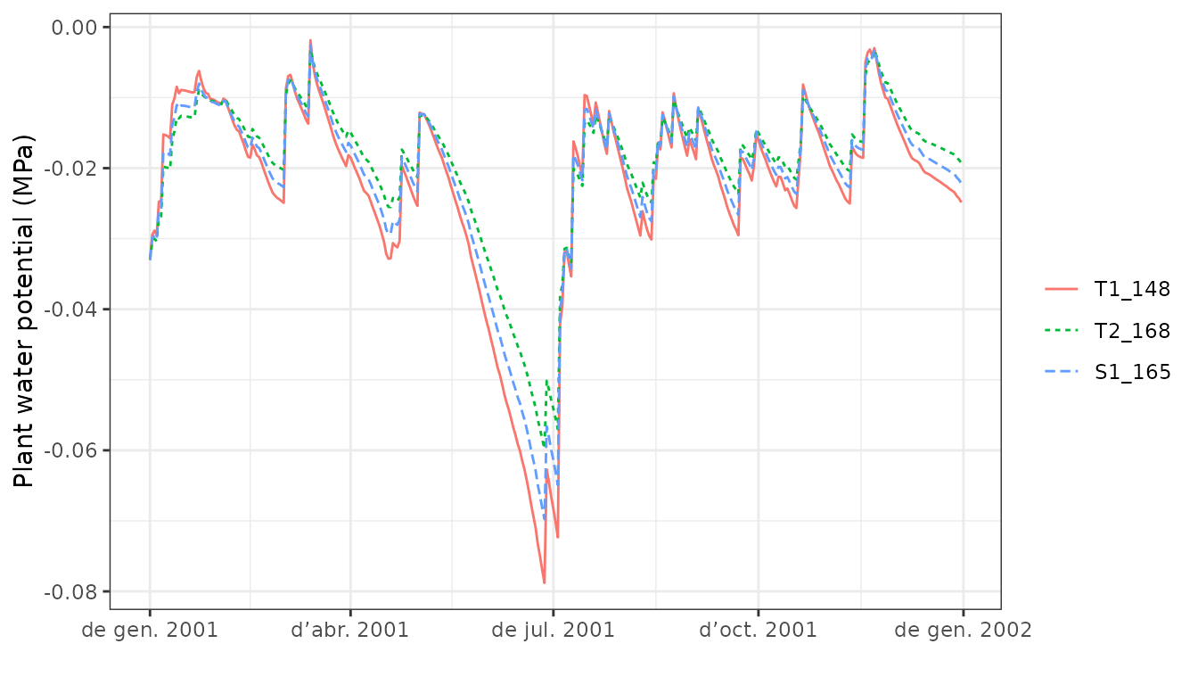

Finally, one can interactively create plots using function shinyplot, e.g.:

shinyplot(S)

Extracting output

Simulation outputs in form of lists have a nested structure that is not easy to handle. Functions are provided to extract model outputs as data.frame objects. The following code extracts daily series of stand-level variables:

df <- extract(S, "forest")
head(df)

##         date       PET Precipitation      Rain Snow    NetRain Snowmelt
## 1 2001-01-01 0.8828475      4.869109  4.869109    0  3.4241795        0
## 2 2001-01-02 1.6375337      2.498292  2.498292    0  1.0717469        0
## 3 2001-01-03 1.3017026      0.000000  0.000000    0  0.0000000        0
## 4 2001-01-04 0.5690790      5.796973  5.796973    0  4.3625616        0
## 5 2001-01-05 1.6760567      1.884401  1.884401    0  0.7539027        0
## 6 2001-01-06 1.2077028     13.359801 13.359801    0 11.7240275        0
##   Infiltration InfiltrationExcess SaturationExcess Runoff DeepDrainage
## 1    3.4241795                  0                0      0  0.005453485
## 2    1.0717469                  0                0      0  0.005216676
## 3    0.0000000                  0                0      0  0.005017641
## 4    4.3625616                  0                0      0  0.005200701
## 5    0.7539027                  0                0      0  0.005869696
## 6   11.7240275                  0                0      0  0.005890970
##   CapillarityRise Evapotranspiration Interception SoilEvaporation
## 1    4.316996e-05          2.0551277     1.444929      0.44789475
## 2    1.894436e-05          1.7950032     1.426545      0.06716959
## 3    0.000000e+00          0.2959936     0.000000      0.05645746
## 4    3.170545e-04          1.6060978     1.434411      0.06697917
## 5    0.000000e+00          1.4656495     1.130499      0.02644820
## 6    4.331022e-03          1.8842477     1.635773      0.02602566
##   HerbTranspiration PlantExtraction Transpiration HydraulicRedistribution
## 1       0.011023432      0.15128020    0.15128020             0.000000000
## 2       0.020448154      0.28084078    0.28084078             0.017679718
## 3       0.016254782      0.22328135    0.22328135             0.014393466
## 4       0.007106185      0.09760108    0.09760108             0.006500031
## 5       0.020931015      0.28777147    0.28777147             0.019396272
## 6       0.015082123      0.20736677    0.20736677             0.014283588
##        LAI   LAIherb  LAIlive LAIexpanded LAIdead       Cm LgroundPAR
## 1 1.758585 0.1736369 1.584948    1.584948       0 1.390485   40.00754
## 2 1.758585 0.1736369 1.584948    1.584948       0 1.390485   40.00754
## 3 1.758585 0.1736369 1.584948    1.584948       0 1.390485   40.00754
## 4 1.758585 0.1736369 1.584948    1.584948       0 1.390485   40.00754
## 5 1.758585 0.1736369 1.584948    1.584948       0 1.390485   40.00754
## 6 1.758585 0.1736369 1.584948    1.584948       0 1.390485   40.00754
##   LgroundSWR      W.1      W.2      W.3      W.4     ML.1     ML.2     ML.3
## 1   50.73297 1.000000 1.000000 1.000000 1.000000 68.17381 116.6530 75.74868
## 2   50.73297 1.026805 1.007621 1.000976 1.000603 70.00119 117.5420 75.82263
## 3   50.73297 1.032063 1.009865 1.001655 1.001475 70.35964 117.8038 75.87406
## 4   50.73297 1.026884 1.009796 1.002130 1.002272 70.00658 117.7956 75.91006
## 5   50.73297 1.069132 1.019944 1.003429 1.003048 72.88681 118.9795 76.00845
## 6   50.73297 1.070261 1.022050 1.004237 1.004009 72.96375 119.2251 76.06961
##       ML.4    MLTot SaturatedDepth SWE PlantExt.1 PlantExt.2   PlantExt.3
## 1 30.29947 290.8749       3960.953   0 0.11011216 0.03647462  0.003757603
## 2 30.31773 293.6835       3946.970   0 0.24012871 0.05839178 -0.006336220
## 3 30.34415 294.3816       3945.796   0 0.19179936 0.04587546 -0.005379180
## 4 30.36831 294.0806       3888.998   0 0.08318975 0.02091136 -0.002505371
## 5 30.39183 298.2666       3877.596   0 0.25639492 0.05077282 -0.007773092
## 6 30.42095 298.6795       3728.041   0 0.18452196 0.03712840 -0.005791528
##      PlantExt.4 HydraulicInput.1 HydraulicInput.2 HydraulicInput.3
## 1  0.0009358264                0                0      0.000000000
## 2 -0.0113434982                0                0      0.006336220
## 3 -0.0090142857                0                0      0.005379180
## 4 -0.0039946606                0                0      0.002505371
## 5 -0.0116231800                0                0      0.007773092
## 6 -0.0084920601                0                0      0.005791528
##   HydraulicInput.4       psi.1       psi.2       psi.3       psi.4
## 1      0.000000000 -0.02905801 -0.03182940 -0.03284772 -0.03290592
## 2      0.011343498 -0.02833948 -0.03149249 -0.03274222 -0.03277025
## 3      0.009014286 -0.02904709 -0.03150287 -0.03266857 -0.03264667
## 4      0.003994661 -0.02371706 -0.03002147 -0.03246809 -0.03252681
## 5      0.011623180 -0.02358750 -0.02972257 -0.03234409 -0.03237897
## 6      0.008492060 -0.01290021 -0.02596168 -0.03189963 -0.03222651

And a similar code can be used to daily series of cohort-level variables:

df <- extract(S, "cohort")
head(df)

##         date cohort          species       LAI   LAIlive     FPAR
## 1 2001-01-01 T1_148 Pinus halepensis 0.8487477 0.8487477 92.18285
## 2 2001-01-02 T1_148 Pinus halepensis 0.8487477 0.8487477 92.18285
## 3 2001-01-03 T1_148 Pinus halepensis 0.8487477 0.8487477 92.18285
## 4 2001-01-04 T1_148 Pinus halepensis 0.8487477 0.8487477 92.18285
## 5 2001-01-05 T1_148 Pinus halepensis 0.8487477 0.8487477 92.18285
## 6 2001-01-06 T1_148 Pinus halepensis 0.8487477 0.8487477 92.18285
##   AbsorbedSWRFraction Transpiration GrossPhotosynthesis    PlantPsi     LeafPLC
## 1            35.07634    0.09247256           0.8934407 -0.03300000 0.003069557
## 2            35.07634    0.17167412           1.5611935 -0.02947344 0.002505289
## 3            35.07634    0.13648859           1.3089814 -0.02881534 0.002403213
## 4            35.07634    0.05966133           0.5973071 -0.02941957 0.002496895
## 5            35.07634    0.17591142           1.6201559 -0.02469534 0.001848979
## 6            35.07634    0.12675944           1.3122096 -0.02454389 0.001766723
##   StemPLC PlantWaterBalance   LeafRWC   StemRWC     LFMC PlantStress
## 1       0      0.000000e+00 0.9979679 0.9998350 125.8900 0.005808769
## 2       0      1.932582e-04 0.9981850 0.9998526 125.9051 0.004921478
## 3       0      3.606612e-05 0.9982255 0.9998559 125.9079 0.004761109
## 4       0     -3.311383e-05 0.9981883 0.9998529 125.9053 0.004908287
## 5       0      2.589163e-04 0.9984791 0.9998765 125.9254 0.003796424
## 6       0      8.300658e-06 0.9984884 0.9998772 125.9260 0.003762299

Temporal summaries

While the simulation model uses daily steps, users will normally be interested in outputs at larger time scales. The package provides a summary for objects of class spwb. This function can be used to summarize the model’s output at different temporal steps (i.e. weekly, annual, …). For example, to obtain the average soil moisture and water potentials by months one can use:

summary(S, freq="months",FUN=mean, output="Soil")

##                  W.1      W.2      W.3      W.4     ML.1     ML.2      ML.3
## 2001-01-01 1.2134548 1.125449 1.023824 1.009412 82.72584 131.2870  77.55334
## 2001-02-01 1.1347381 1.212487 1.149547 1.067065 77.35942 141.4402  87.07665
## 2001-03-01 1.1925754 1.259497 1.296163 1.296357 81.30241 146.9241  98.18264
## 2001-04-01 1.0522992 1.168234 1.267811 1.374344 71.73925 136.2779  96.03500
## 2001-05-01 1.0775631 1.157910 1.234312 1.347063 73.46158 135.0737  93.49752
## 2001-06-01 0.8822998 1.038523 1.161615 1.283609 60.14974 121.1468  87.99081
## 2001-07-01 1.1117691 1.100933 1.127050 1.210947 75.79354 128.4271  85.37255
## 2001-08-01 1.1103916 1.167904 1.208133 1.282990 75.69963 136.2395  91.51449
## 2001-09-01 1.1033174 1.179468 1.248817 1.354485 75.21735 137.5885  94.59623
## 2001-10-01 1.1263208 1.176821 1.238020 1.350389 76.78559 137.2796  93.77838
## 2001-11-01 1.1744510 1.234944 1.288074 1.370818 80.06681 144.0599  97.56987
## 2001-12-01 1.0956171 1.224555 1.330559 1.392130 74.69240 142.8480 100.78806
##                ML.4    MLTot SaturatedDepth        SWE PlantExt.1 PlantExt.2
## 2001-01-01 30.58465 322.1508      3484.6231 1.65619239  0.1547078 0.03340906
## 2001-02-01 32.33150 338.2077      2791.7151 0.27608905  0.2405996 0.15753606
## 2001-03-01 39.27895 365.6881      1109.7159 0.01762496  0.2370478 0.12913424
## 2001-04-01 41.64189 345.6941      1133.6514 0.58072652  0.2475781 0.17879922
## 2001-05-01 40.81531 342.8481      1340.4006 0.00000000  0.3117004 0.19939679
## 2001-06-01 38.89268 308.1801      2130.3377 0.00000000  0.2723951 0.37623450
## 2001-07-01 36.69106 326.2843      2324.7625 0.00000000  0.5214002 0.16657848
## 2001-08-01 38.87392 342.3275      1654.9210 0.00000000  0.4349136 0.21601386
## 2001-09-01 41.04018 348.4422      1202.3767 0.00000000  0.3180741 0.17459060
## 2001-10-01 40.91608 348.7597      1234.9718 0.00000000  0.2386751 0.10806618
## 2001-11-01 41.53506 363.2317       848.0663 2.60802857  0.1671801 0.08579823
## 2001-12-01 42.18081 360.5092       752.0311 0.00000000  0.1286244 0.09571566
##              PlantExt.3   PlantExt.4 HydraulicInput.1 HydraulicInput.2
## 2001-01-01 -0.005833200 -0.008206203                0      0.000000000
## 2001-02-01  0.014680002 -0.020651145                0      0.000000000
## 2001-03-01  0.029294705  0.012466026                0      0.000000000
## 2001-04-01  0.050545209  0.053505279                0      0.000000000
## 2001-05-01  0.052468212  0.065684214                0      0.000000000
## 2001-06-01  0.129447741  0.119158903                0      0.000000000
## 2001-07-01  0.009688123  0.065513395                0      0.001533827
## 2001-08-01  0.044897710  0.071917231                0      0.000000000
## 2001-09-01  0.042773582  0.058735615                0      0.000000000
## 2001-10-01  0.025527544  0.041652261                0      0.000000000
## 2001-11-01  0.016505039  0.026081213                0      0.000000000
## 2001-12-01  0.028585552  0.023755251                0      0.000000000
##            HydraulicInput.3 HydraulicInput.4       psi.1        psi.2
## 2001-01-01     5.954413e-03      0.008236391 -0.01142747 -0.018363087
## 2001-02-01     2.273595e-03      0.020651145 -0.01810497 -0.011254552
## 2001-03-01     5.630267e-04      0.007556396 -0.01293057 -0.008053885
## 2001-04-01     0.000000e+00      0.000000000 -0.02629300 -0.014540879
## 2001-05-01     0.000000e+00      0.000000000 -0.02468247 -0.015360169
## 2001-06-01     0.000000e+00      0.000000000 -0.05976539 -0.028336401
## 2001-07-01     1.856098e-02      0.000000000 -0.02134239 -0.020875506
## 2001-08-01     4.894657e-04      0.000000000 -0.02006077 -0.014356494
## 2001-09-01     0.000000e+00      0.000000000 -0.02046436 -0.013528880
## 2001-10-01     3.897806e-05      0.000000000 -0.01849177 -0.013647653
## 2001-11-01     2.540720e-03      0.000000000 -0.01489545 -0.009744551
## 2001-12-01     0.000000e+00      0.000000000 -0.02144571 -0.010468175
##                   psi.3        psi.4
## 2001-01-01 -0.029328778 -0.031476171
## 2001-02-01 -0.015672673 -0.023832141
## 2001-03-01 -0.005867455 -0.005776684
## 2001-04-01 -0.007741972 -0.001702982
## 2001-05-01 -0.009679389 -0.003242426
## 2001-06-01 -0.015175039 -0.006887816
## 2001-07-01 -0.017691899 -0.011145942
## 2001-08-01 -0.011252055 -0.006525493
## 2001-09-01 -0.008718190 -0.002778769
## 2001-10-01 -0.009338631 -0.003008966
## 2001-11-01 -0.006252047 -0.001737364
## 2001-12-01 -0.004219673 -0.000565659

Parameter output is used to indicate the element of the spwb object for which we desire summaries. Similarly, it is possible to calculate the average stress of plant cohorts by months:

summary(S, freq="months",FUN=mean, output="PlantStress")

##                 T1_148      T2_168       S1_165
## 2001-01-01 0.001744444 0.005022187 0.0011740571
## 2001-02-01 0.002222738 0.004495608 0.0012113811
## 2001-03-01 0.001483256 0.003185728 0.0008167336
## 2001-04-01 0.003793490 0.006218154 0.0018614834
## 2001-05-01 0.003544500 0.006060525 0.0017705291
## 2001-06-01 0.012368214 0.014020890 0.0052048056
## 2001-07-01 0.003829278 0.006961042 0.0019801381
## 2001-08-01 0.002739974 0.005303452 0.0014512601
## 2001-09-01 0.002735561 0.005173780 0.0014303118
## 2001-10-01 0.002378301 0.004864224 0.0012901214
## 2001-11-01 0.001874120 0.003763899 0.0010017251
## 2001-12-01 0.002735117 0.004735996 0.0013706938

The summary function can be also used to aggregate the output by species. In this case, the values of plant cohorts belonging to the same species will be averaged using LAI values as weights. For example, we may average the daily drought stress across cohorts of the same species (here there is only one cohort by species, so this does not modify the output):

head(summary(S, freq="day", output="PlantStress", bySpecies = TRUE))

##            Pinus halepensis Quercus coccifera Quercus ilex
## 2001-01-01      0.005808769       0.003088161  0.010612890
## 2001-01-02      0.004921478       0.002728995  0.009760353
## 2001-01-03      0.004761109       0.002660356  0.009585196
## 2001-01-04      0.004908287       0.002716293  0.009705299
## 2001-01-05      0.003796424       0.002255203  0.008577056
## 2001-01-06      0.003762299       0.002235134  0.008507586

Or we can combine the aggregation by species with a temporal aggregation (here monthly averages):

summary(S, freq="month", FUN = mean, output="PlantStress", bySpecies = TRUE)

##            Pinus halepensis Quercus coccifera Quercus ilex
## 2001-01-01      0.001744444      0.0011740571  0.005022187
## 2001-02-01      0.002222738      0.0012113811  0.004495608
## 2001-03-01      0.001483256      0.0008167336  0.003185728
## 2001-04-01      0.003793490      0.0018614834  0.006218154
## 2001-05-01      0.003544500      0.0017705291  0.006060525
## 2001-06-01      0.012368214      0.0052048056  0.014020890
## 2001-07-01      0.003829278      0.0019801381  0.006961042
## 2001-08-01      0.002739974      0.0014512601  0.005303452
## 2001-09-01      0.002735561      0.0014303118  0.005173780
## 2001-10-01      0.002378301      0.0012901214  0.004864224
## 2001-11-01      0.001874120      0.0010017251  0.003763899
## 2001-12-01      0.002735117      0.0013706938  0.004735996

Specific output functions

The package provides some functions to extract or transform specific outputs from soil plant water balance simulations. In particular, function droughtStress() allows calculating several plant stress indices, such as the number of days with drought stress > 0.5 or the maximum drought stress:

droughtStress(S, index = "NDD", freq = "years", draw=FALSE)

##            T1_148 T2_168 S1_165
## 2001-01-01      0      0      0

droughtStress(S, index = "MDS", freq = "years", draw=FALSE)

##                T1_148     T2_168      S1_165
## 2001-01-01 0.01818643 0.01843434 0.007314233

As the general summary function, droughtStress() allows calculating stress indices at several temporal scales. For example the water stress index (integral of water potential values) can be calculated and drawn for every month:

droughtStress(S, index = "WSI", freq = "months", draw=TRUE)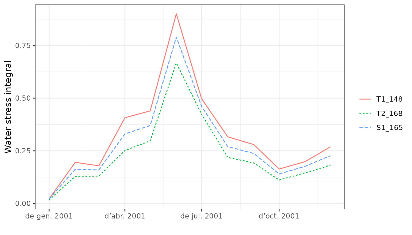

Another specific summary function is waterUseEfficiency(). This is most useful with advanced water and energy balance modeling, but for simple water balance it calculates the ratio between photosynthesis and transpiration at the desired scale. In this case it is equal to the value of the input species parameter WUE:

waterUseEfficiency(S, type = "Stand Ag/E", freq = "months", draw=FALSE)

##            Stand Ag/E
## 2001-01-01  10.040831
## 2001-02-01   8.179078
## 2001-03-01   8.977419
## 2001-04-01   8.807673
## 2001-05-01   8.207497
## 2001-06-01   6.284423
## 2001-07-01   6.966492
## 2001-08-01   6.219283
## 2001-09-01   7.434574
## 2001-10-01   7.643271
## 2001-11-01   8.711049
## 2001-12-01   8.406632

References

De Cáceres M, Martínez-Vilalta J, Coll L, Llorens P, Casals P, Poyatos R, Pausas JG, Brotons L. (2015) Coupling a water balance model with forest inventory data to predict drought stress: the role of forest structural changes vs. climate changes. Agricultural and Forest Meteorology 213: 77-90 (https://doi.org/10.1016/j.agrformet.2015.06.012).

Miquel De Caceres

2024-04-16