Advanced water and energy balance

About this vignette

This document describes how to run a water and energy balance model that uses a more detailed approach for hydraulics and stomatal regulation described in De Cáceres et al. (2021) and Ruffault et al. (2022). We recommend reading vignette Basic water balance before this one for a more accessible introduction to soil water balance modelling. This vignette is meant to teach users to run the simulation model within R. All the details of the model design and formulation can be found at the medfatebook.

Preparing model inputs

Model inputs are explained in greater detail in vignettes Understanding model inputs and Preparing model inputs. Here we only review the different steps required to run function spwb().

Soil, vegetation, meteorology and species data

Soil information needs to be entered as a data frame with soil layers in rows and physical attributes in columns. Soil physical attributes can be initialized to default values, for a given number of layers, using function defaultSoilParams():

spar <- defaultSoilParams(4)

The soil input for water balance simulation is actually a list of class soil that is created using a function with the same name:

examplesoil <- soil(spar)

As explained in the package overview, models included in medfate were primarily designed to be ran on forest inventory plots. Here we use the example object provided with the package:

data(exampleforest)
exampleforest

## $treeData
##            Species   N   DBH Height Z50  Z95
## 1 Pinus halepensis 168 37.55    800 100  600
## 2     Quercus ilex 384 14.60    660 300 1000
## 
## $shrubData
##             Species Cover Height Z50  Z95
## 1 Quercus coccifera  3.75     80 200 1000
## 
## $herbCover
## [1] 10
## 
## $herbHeight
## [1] 20
## 
## $seedBank
## [1] Species Percent
## <0 rows> (or 0-length row.names)
## 
## attr(,"class")
## [1] "forest" "list"

Importantly, a data frame with daily weather for the period to be simulated is required. Here we use the default data frame included with the package:

data(examplemeteo)
head(examplemeteo)

##        dates MinTemperature MaxTemperature Precipitation MinRelativeHumidity
## 1 2001-01-01     -0.5934215       6.287950      4.869109            65.15411
## 2 2001-01-02     -2.3662458       4.569737      2.498292            57.43761
## 3 2001-01-03     -3.8541036       2.661951      0.000000            58.77432
## 4 2001-01-04     -1.8744860       3.097705      5.796973            66.84256
## 5 2001-01-05      0.3288287       7.551532      1.884401            62.97656
## 6 2001-01-06      0.5461322       7.186784     13.359801            74.25754
##   MaxRelativeHumidity Radiation WindSpeed
## 1           100.00000  12.89251  2.000000
## 2            94.71780  13.03079  7.662544
## 3            94.66823  16.90722  2.000000
## 4            95.80950  11.07275  2.000000
## 5           100.00000  13.45205  7.581347
## 6           100.00000  12.84841  6.570501

Finally, simulations in medfate require a data frame with species parameter values, which we load using defaults for Catalonia (NE Spain):

data("SpParamsMED")

Simulation control

Apart from data inputs, the behaviour of simulation models is controlled using a set of global parameters. The default parameterization is obtained using function defaultControl():

control <- defaultControl("Sperry")

To use the advanced water balance model we must change the values of transpirationMode to switch from "Granier" to either "Sperry" or "Sureau".

Water balance input object

A last object is needed before calling simulation functions, called spwbInput. It consists in the compilation of aboveground, belowground parameters and the specification of additional parameter values for each plant cohort. This is done by calling function forest2spwbInput():

x <- forest2spwbInput(exampleforest, examplesoil, SpParamsMED, control)

The spwbInput object for advanced water and energy balance is similar to that of simple water balance simulations, but contains more elements. Information about the cohort species is found in element cohorts, i.e. the cohort code, the species index and species name:

x$cohorts

##         SP              Name
## T1_148 148  Pinus halepensis
## T2_168 168      Quercus ilex
## S1_165 165 Quercus coccifera

Element canopy contains state variables within the canopy:

x$canopy

##    zlow zmid  zup Tair Cair VPair
## 1     0   50  100   NA   NA    NA
## 2   100  150  200   NA   NA    NA
## 3   200  250  300   NA   NA    NA
## 4   300  350  400   NA   NA    NA
## 5   400  450  500   NA   NA    NA
## 6   500  550  600   NA   NA    NA
## 7   600  650  700   NA   NA    NA
## 8   700  750  800   NA   NA    NA
## 9   800  850  900   NA   NA    NA
## 10  900  950 1000   NA   NA    NA
## 11 1000 1050 1100   NA   NA    NA
## 12 1100 1150 1200   NA   NA    NA
## 13 1200 1250 1300   NA   NA    NA
## 14 1300 1350 1400   NA   NA    NA
## 15 1400 1450 1500   NA   NA    NA
## 16 1500 1550 1600   NA   NA    NA
## 17 1600 1650 1700   NA   NA    NA
## 18 1700 1750 1800   NA   NA    NA
## 19 1800 1850 1900   NA   NA    NA
## 20 1900 1950 2000   NA   NA    NA
## 21 2000 2050 2100   NA   NA    NA
## 22 2100 2150 2200   NA   NA    NA
## 23 2200 2250 2300   NA   NA    NA
## 24 2300 2350 2400   NA   NA    NA
## 25 2400 2450 2500   NA   NA    NA
## 26 2500 2550 2600   NA   NA    NA
## 27 2600 2650 2700   NA   NA    NA
## 28 2700 2750 2800   NA   NA    NA

Canopy temperature, water vapour pressure and $CO_2$ concentration are state variables needed for canopy energy balance. If the canopy energy balance assumes a single canopy layer, the same values will be assumed through the canopy. Variation of within-canopy state variables is modelled if a multi-canopy energy balance is used (see control parameter multiLayerBalance).

As you may already known, element above contains the aboveground structure data that we already know:

x$above

##          H        CR   LAI_live LAI_expanded LAI_dead
## T1_148 800 0.6605196 0.84874773   0.84874773        0
## T2_168 660 0.6055642 0.70557382   0.70557382        0
## S1_165  80 0.8032817 0.03062604   0.03062604        0

Belowground parameters can be seen in below:

x$below

##        Z50  Z95
## T1_148 100  600
## T2_168 300 1000
## S1_165 200 1000

and in belowLayers:

x$belowLayers

## $V
##                1         2          3           4
## T1_148 0.8604899 0.1194556 0.01511005 0.004944476
## T2_168 0.5008953 0.4505941 0.04064831 0.007862284
## S1_165 0.6799879 0.2737911 0.03567632 0.010544678
## 
## $L
##               1        2        3        4
## T1_148 2289.062 1566.552 2250.052 4226.166
## T2_168 1817.571 2100.346 2410.127 4285.194
## S1_165 1085.030 1380.808 2170.587 4146.637
## 
## $VGrhizo_kmax
##                 1           2           3          4
## T1_148   296483.4    41158.65    5206.196   1703.629
## T2_168 46380598.9 41722941.01 3763846.755 728011.313
## S1_165 10941458.6  4405482.18  574055.729 169670.901
## 
## $VCroot_kmax
##               1         2          3           4
## T1_148 2.382795 0.4833484 0.04256689 0.007416044
## T2_168 1.568929 1.2213562 0.09601747 0.010445417
## S1_165 2.407779 0.7618041 0.06314806 0.009770000
## 
## $Wpool
##        1 2 3 4
## T1_148 1 1 1 1
## T2_168 1 1 1 1
## S1_165 1 1 1 1
## 
## $RhizoPsi
##             1      2      3      4
## T1_148 -0.033 -0.033 -0.033 -0.033
## T2_168 -0.033 -0.033 -0.033 -0.033
## S1_165 -0.033 -0.033 -0.033 -0.033

The spwbInputobject also includes cohort parameter values for several kinds of traits. For example, plant anatomy parameters are described in paramsAnatomy:

x$paramsAnatomy

##        Hmed    Al2As      SLA LeafWidth LeafDensity WoodDensity FineRootDensity
## T1_148  850 1317.523 5.140523 0.1384772   0.2982842   0.6077016       0.2982842
## T2_168  500 3908.823 6.340000 1.7674359   0.4893392   0.9008264       0.4893392
## S1_165   80 4189.325 4.980084 1.3761085   0.3709679   0.4389106       0.3709679
##        conduit2sapwood      SRL RLD     r635
## T1_148       0.9236406 3172.572  10 1.964226
## T2_168       0.6238125 4398.812  10 1.805872
## S1_165       0.6238125 4398.812  10 2.289452

Parameters related to plant transpiration and photosynthesis can be seen in paramsTranspiration:

x$paramsTranspiration

##             Gswmin    Gswmax  Vmax298  Jmax298 Kmax_stemxylem Kmax_rootxylem
## T1_148 0.003086667 0.2850000 72.19617 124.1687           0.15           0.60
## T2_168 0.004473333 0.2007222 68.51600 118.7863           0.40           1.60
## S1_165 0.010455247 0.2830167 62.78100 118.4486           0.29           1.16
##        VCleaf_kmax VCleafapo_kmax VCleaf_c  VCleaf_d kleaf_symp VCstem_kmax
## T1_148    4.000000        8.00000 1.456324 -1.536975    8.00000    1.339563
## T2_168    4.000000        8.00000 2.254991 -3.133381    8.00000    1.620936
## S1_165    9.579077       19.15815 2.254991 -3.133381   19.15815    4.599269
##        VCstem_c  VCstem_d VCroot_kmax VCroot_c   VCroot_d VGrhizo_kmax
## T1_148 5.030852 -4.797531    2.916127 3.193056 -0.9870357     344551.9
## T2_168 2.731881 -4.278250    2.896748 1.182310 -2.5041509   92595397.9
## S1_165 3.095442 -7.857378    3.242501 1.402489 -1.5233241   16090667.4
##        Plant_kmax   FR_leaf   FR_stem   FR_root
## T1_148  0.7465846 0.1866462 0.5573346 0.2560193
## T2_168  0.8249857 0.2062464 0.5089563 0.2847972
## S1_165  1.5867376 0.1656462 0.3449978 0.4893561

Parameters related to pressure-volume curves and water storage capacity of leaf and stem organs are in paramsWaterStorage:

x$paramsWaterStorage

##           maxFMC   LeafPI0   LeafEPS LeafAF     Vleaf   StemPI0   StemEPS
## T1_148 126.03063 -1.591429  8.918571 0.3525 0.5258525 -2.008039 13.256355
## T2_168  93.15304 -1.483333 19.260000 0.1700 0.2199087 -3.227438 46.420610
## S1_165  96.53441 -2.370000 17.230000 0.2400 0.4108968 -1.305868  6.297155
##           StemAF Vsapwood
## T1_148 0.9236406 6.174277
## T2_168 0.6238125 1.278142
## S1_165 0.6238125 1.064511

Finally, remember that one can play with plant-specific parameters for soil water balance (instead of using species-level values) by modifying manually the parameter values in this object.

Static analysis of sub-models

Before using the advanced water and energy balance model, is important to understand the parameters that influence the different sub-models. Package medfate provides low-level functions corresponding to sub-models (light extinction, hydraulics, transpiration, photosynthesis…). In addition, there are several high-level plotting functions that allow examining several aspects of these processes.

Vulnerability curves

Given a spwbInput object, we can use function hydraulics_vulnerabilityCurvePlot() to inspect vulnerability curves (i.e. how hydraulic conductance of a given segment changes with the water potential) for each plant cohort and each of the different segments of the soil-plant hydraulic network: rhizosphere, roots, stems and leaves:

hydraulics_vulnerabilityCurvePlot(x, type="leaf")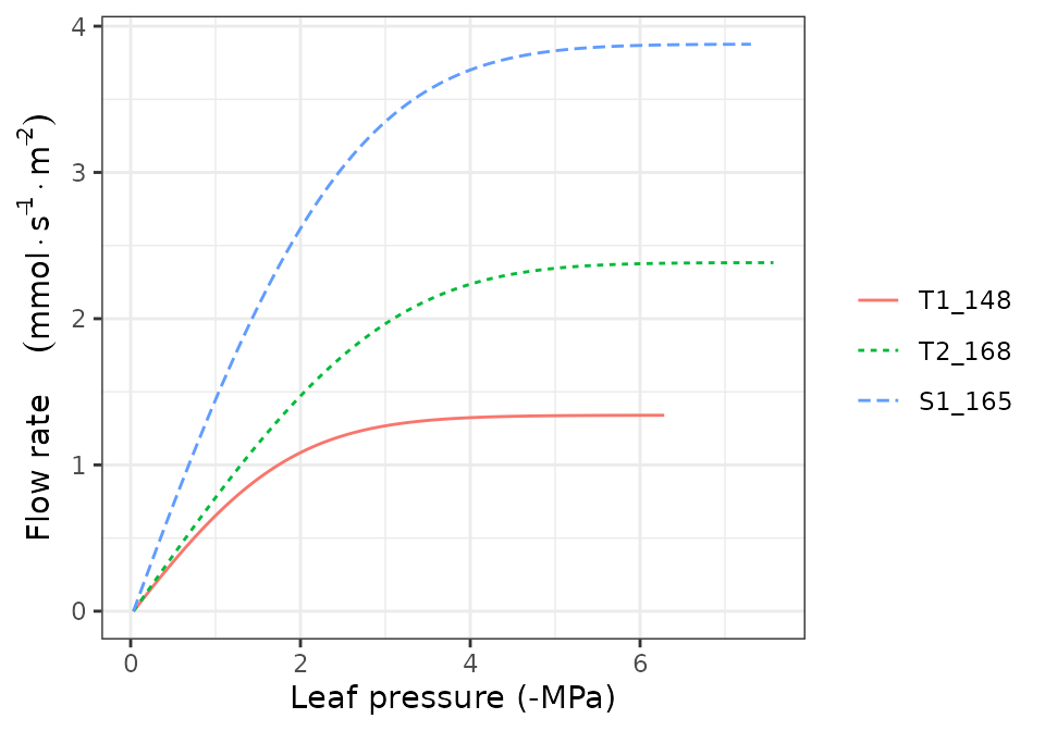

hydraulics_vulnerabilityCurvePlot(x, type="stem")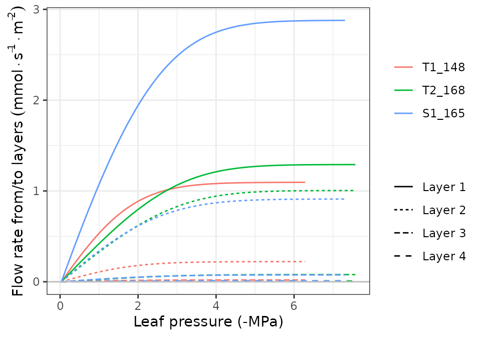

hydraulics_vulnerabilityCurvePlot(x, type="root")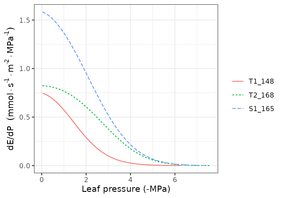

hydraulics_vulnerabilityCurvePlot(x, examplesoil, type="rhizo")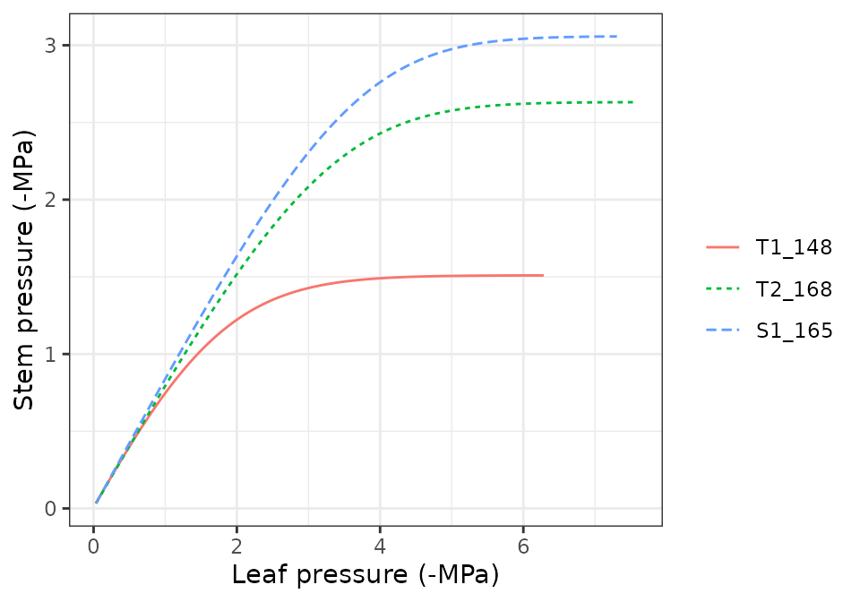

The maximum values and shape of vulnerability curves for leaves and stems are regulated by parameters in paramsTranspiration. Roots have vulnerability curve parameters in the same data frame, but maximum conductance values need to be specified for each soil layer and are given in belowLayers$VCroot_kmax. Note that the last call to hydraulics_vulnerabilityCurvePlot() includes a soil object. This is because the van Genuchten parameters that define the shape of the vulnerability curve for the rhizosphere are stored in this object. Maximum conductance values in the rhizosphere are given in belowLayers$VGrhizo_kmax.

Supply functions

The vulnerability curves conforming the hydraulic network are used in the model to build the supply function, which relates water flow (i.e. transpiration) with the drop of water potential along the whole hydraulic pathway. The supply function contains not only these two variables, but also the water potential of intermediate nodes in the the hydraulic network. Function hydraulics_supplyFunctionPlot() can be used to inspect any of this variables:

hydraulics_supplyFunctionPlot(x, type="E")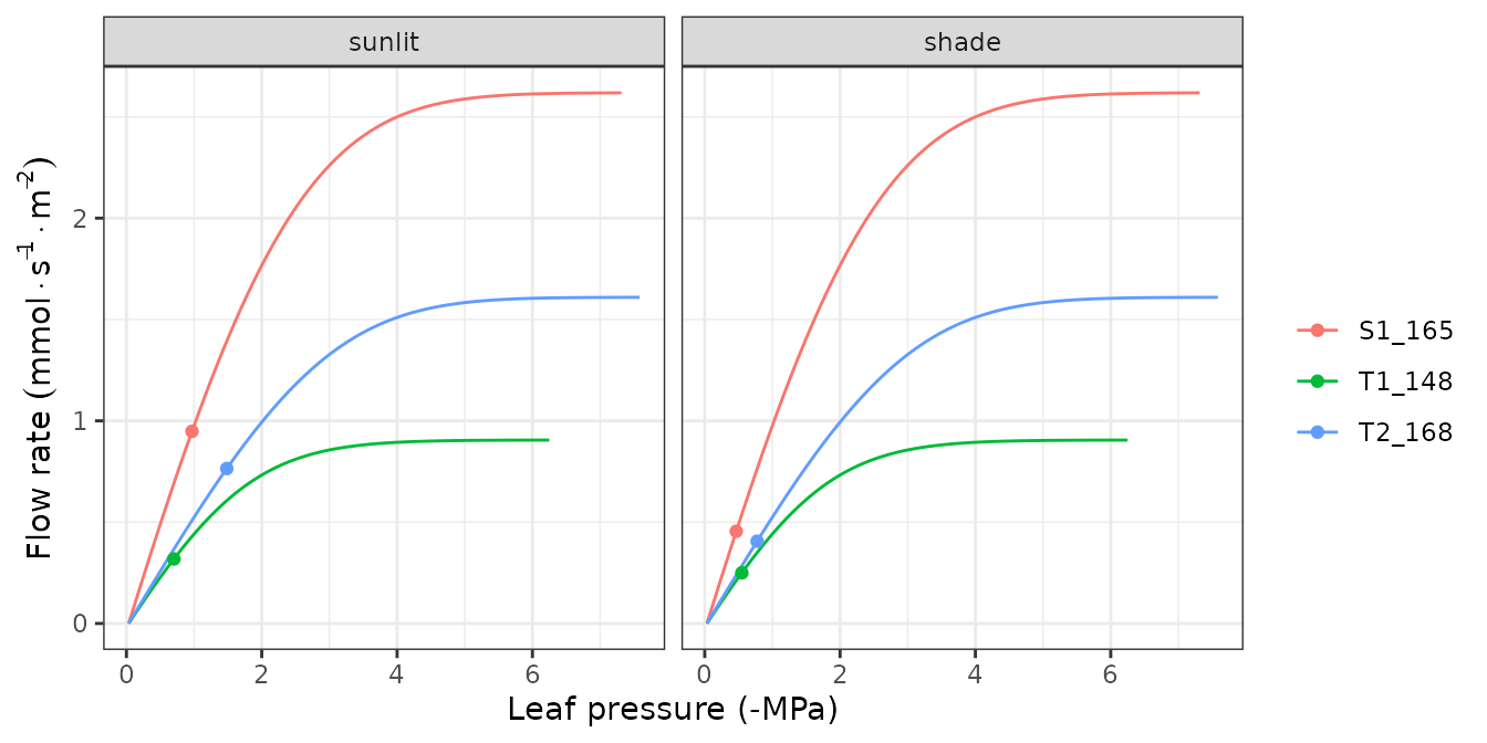

hydraulics_supplyFunctionPlot(x, type="ERhizo")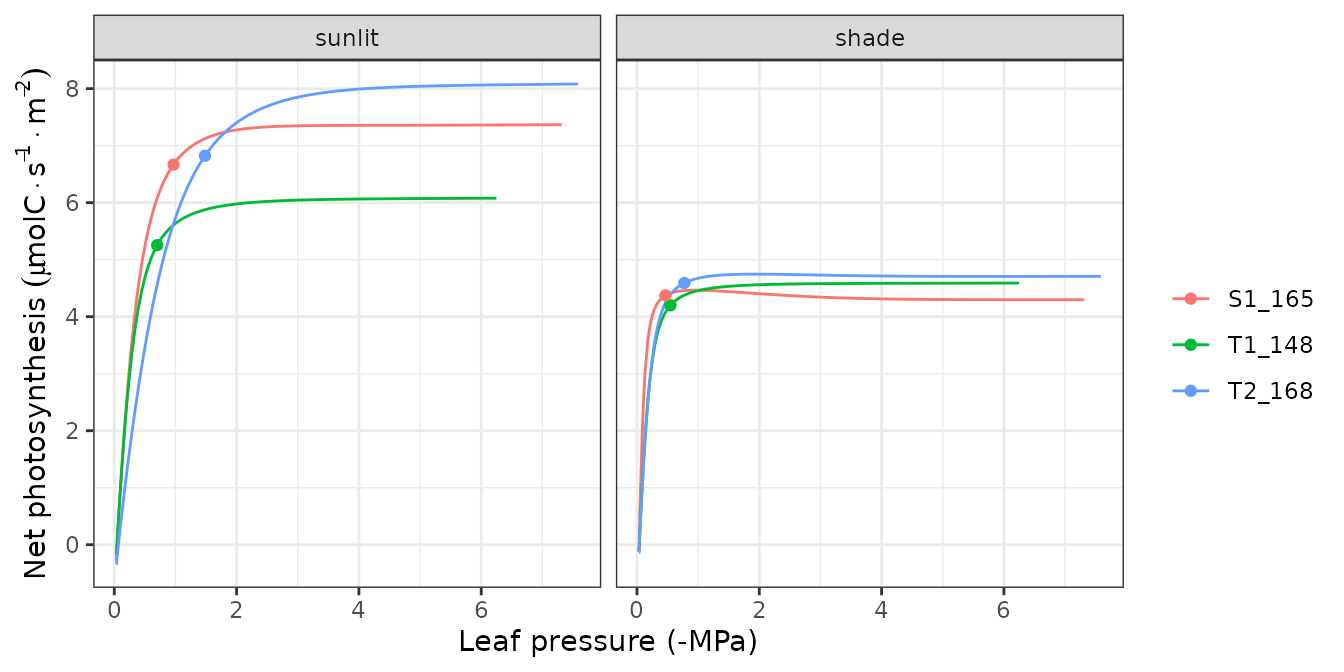

hydraulics_supplyFunctionPlot(x, type="dEdP")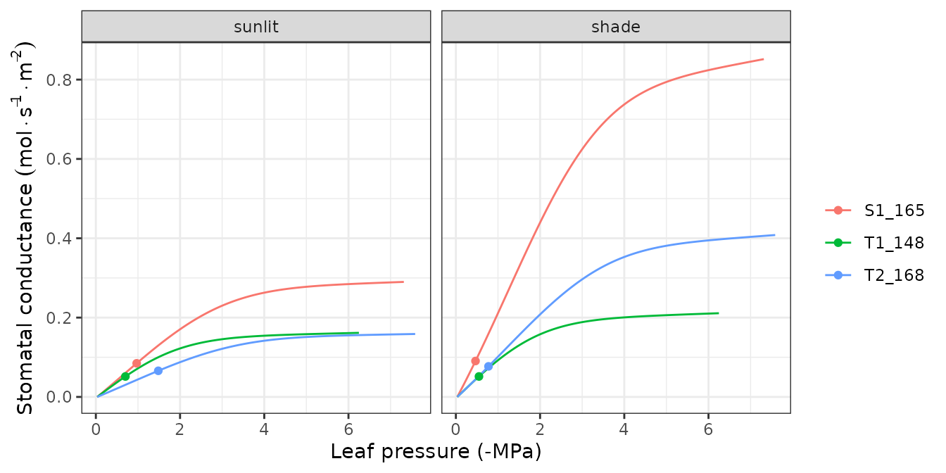

hydraulics_supplyFunctionPlot(x, type="StemPsi")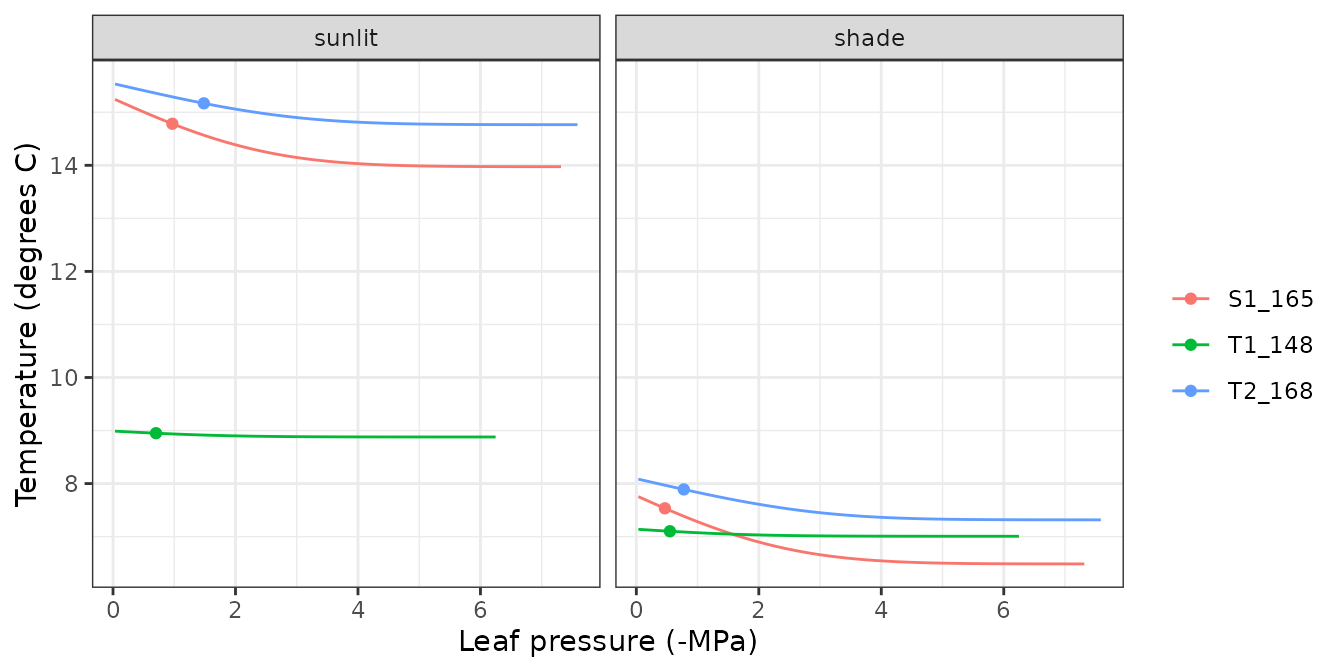

Calls to hydraulics_supplyFunctionPlot() always need both a spwbInput object and a soil object. The soil moisture state (i.e. its water potential) is the starting point for the calculation of the supply function, so different curves will be obtained for different values of soil moisture.

Stomatal regulation and photosynthesis

The soil water balance model determines stomatal conductance and transpiration separately for sunlit and shade leaves. Stomatal conductance is determined after building a photosynthesis function corresponding to the supply function and finding the value of stomatal conductance that maximizes carbon revenue while avoiding hydraulic damage (a profit-maximization approach). Given a meteorological and soil inputs and a chosen day and timestep, function transp_stomatalRegulationPlot() allows displaying the supply and photosynthesis curves for sunlit and shade leaves, along with an indication of the values corresponding to the chosen stomatal aperture:

d <- 100
transp_stomatalRegulationPlot(x, examplemeteo, day = d, timestep=12,
                              latitude = 41.82592, elevation = 100, type="E")

## Package 'meteoland' [ver. 2.2.1]

transp_stomatalRegulationPlot(x, examplemeteo, day = d, timestep=12,
                              latitude = 41.82592, elevation = 100, type="An")

transp_stomatalRegulationPlot(x, examplemeteo, day = d, timestep=12,
                              latitude = 41.82592, elevation = 100, type="Gsw")

transp_stomatalRegulationPlot(x, examplemeteo, day = d, timestep=12,
                              latitude = 41.82592, elevation = 100, type="T")

transp_stomatalRegulationPlot(x, examplemeteo, day = d, timestep=12,
                              latitude = 41.82592, elevation = 100, type="VPD")

Pressure volume curves

moisture_pressureVolumeCurvePlot(x, segment="leaf", fraction="symplastic")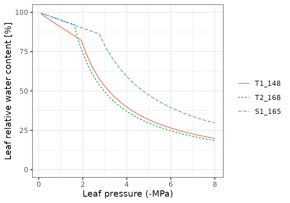

moisture_pressureVolumeCurvePlot(x, segment="leaf", fraction="apoplastic")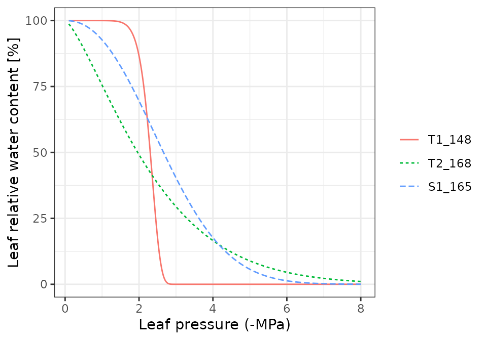

moisture_pressureVolumeCurvePlot(x, segment="stem", fraction="symplastic")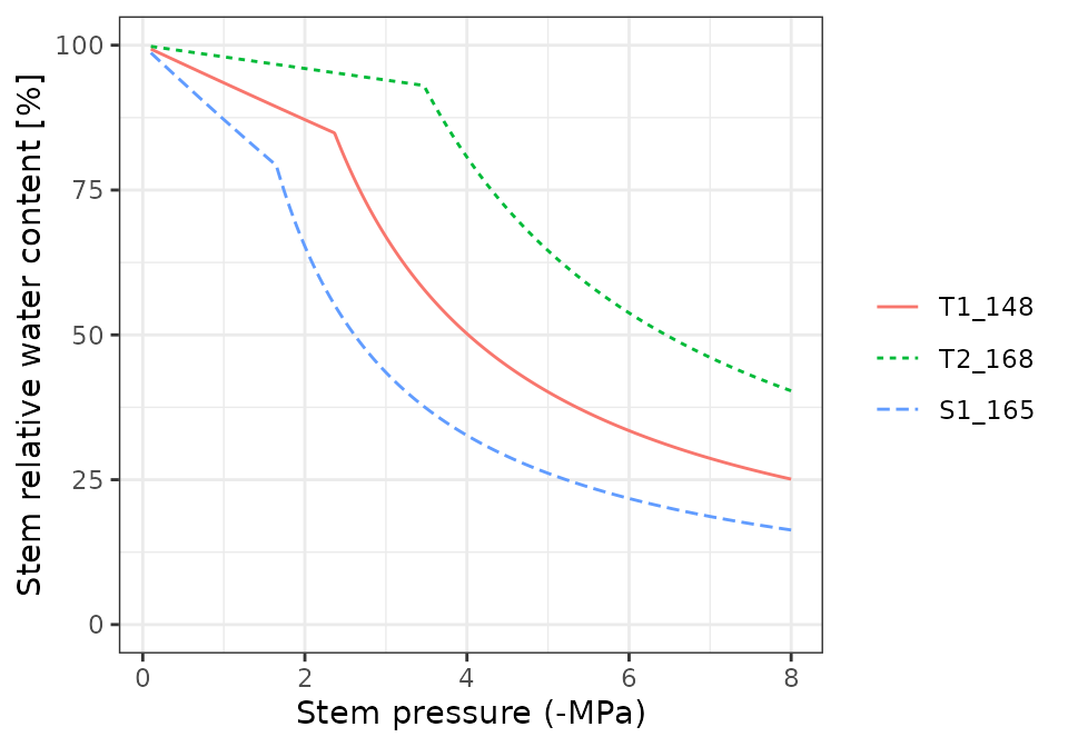

moisture_pressureVolumeCurvePlot(x, segment="stem", fraction="apoplastic")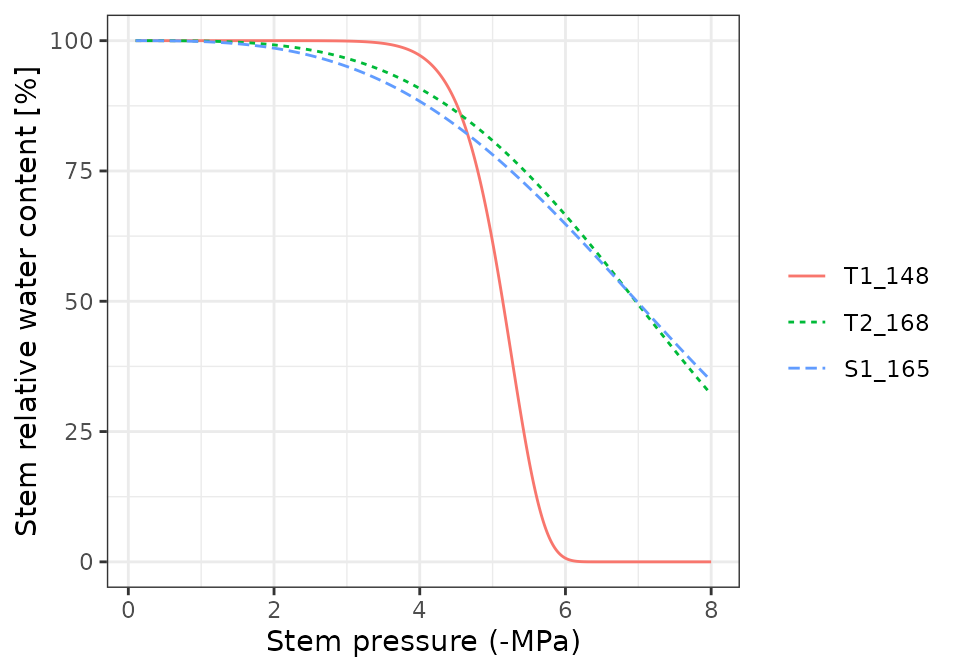

Water balance for a single day

Running the model

Soil water balance simulations will normally span periods of several months or years, but since the model operates at a daily and subdaily temporal scales, it is possible to perform soil water balance for one day only. This is done using function spwb_day(). In the following code we select the same day as before from the meteorological input data and perform soil water balance for that day only:

date <- examplemeteo$dates[d]
meteovec <- unlist(examplemeteo[d,])
sd1<-spwb_day(x, date, meteovec, 
             latitude = 41.82592, elevation = 100, slope= 0, aspect = 0)

The output of spwb_day() is a list with several elements:

names(sd1)

##  [1] "cohorts"          "topography"       "weather"          "WaterBalance"    
##  [5] "EnergyBalance"    "Soil"             "Stand"            "Plants"          
##  [9] "RhizoPsi"         "SunlitLeaves"     "ShadeLeaves"      "ExtractionInst"  
## [13] "PlantsInst"       "SunlitLeavesInst" "ShadeLeavesInst"  "LightExtinction" 
## [17] "LWRExtinction"    "CanopyTurbulence"

Water balance output

Element WaterBalance contains the soil water balance flows of the day (precipitation, infiltration, transpiration, …)

sd1$WaterBalance

##                     PET                    Rain                    Snow 
##            3.902334e+00            0.000000e+00            0.000000e+00 
##                 NetRain                Snowmelt                   Runon 
##            0.000000e+00            0.000000e+00            0.000000e+00 
##            Infiltration      InfiltrationExcess        SaturationExcess 
##            0.000000e+00            0.000000e+00            0.000000e+00 
##                  Runoff            DeepDrainage         CapillarityRise 
##            0.000000e+00            5.243734e-03            1.938321e-05 
##         SoilEvaporation       HerbTranspiration         PlantExtraction 
##            5.000000e-01            4.872542e-02            4.525358e-01 
##           Transpiration HydraulicRedistribution 
##            4.525358e-01            0.000000e+00

And Soil contains water evaporated from each soil layer, water transpired from each soil layer and the final soil water potential:

sd1$Soil

##   HerbTranspiration HydraulicInput HydraulicOutput PlantExtraction         psi
## 1       0.008571001              0     0.295729299     0.295729299 -0.03510522
## 2       0.012000080              0     0.143773933     0.143773933 -0.03317293
## 3       0.013576976              0     0.011591691     0.011591691 -0.03298502
## 4       0.014577363              0     0.001440899     0.001440899 -0.03297440

Soil and canopy energy balance

Element EnergyBalance contains subdaily variation in atmosphere, canopy and soil temperatures, as well as canopy and soil energy balance components.

names(sd1$EnergyBalance)

## [1] "Temperature"         "CanopyEnergyBalance" "SoilEnergyBalance"  
## [4] "TemperatureLayers"   "VaporPressureLayers"

Package medfate provides a plot function for objects of class spwb_day that can be used to inspect the results of the simulation. We use this function to display subdaily dynamics in plant, soil and canopy variables. For example, we can use it to display temperature variations (only the temperature of the topmost soil layer is drawn):

plot(sd1, type = "Temperature")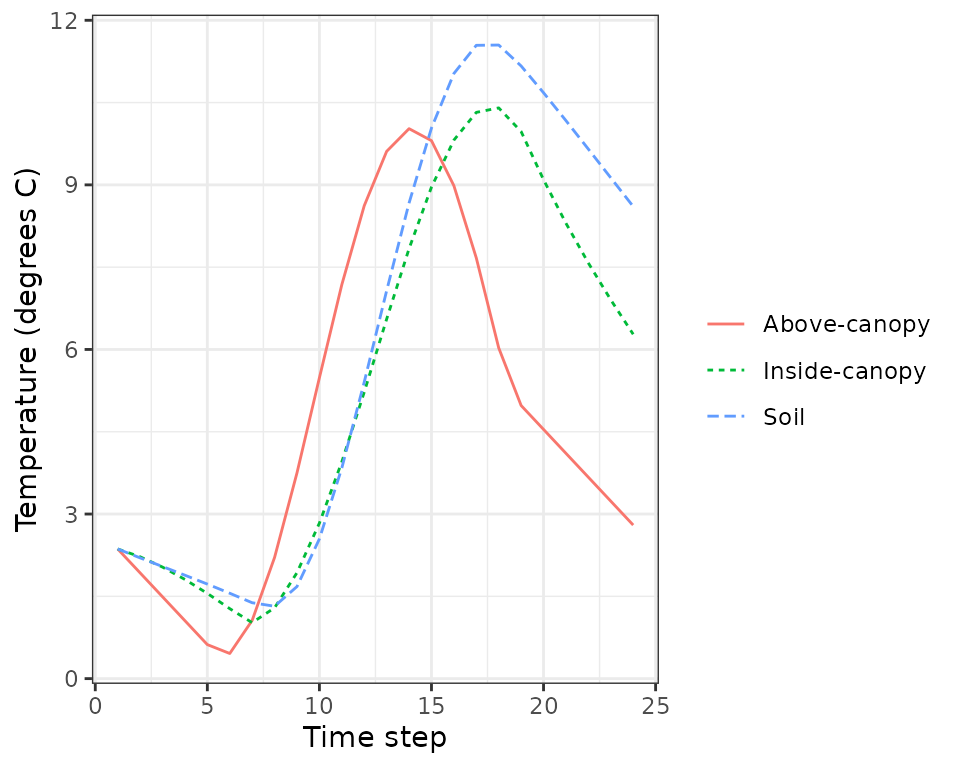

plot(sd1, type = "CanopyEnergyBalance")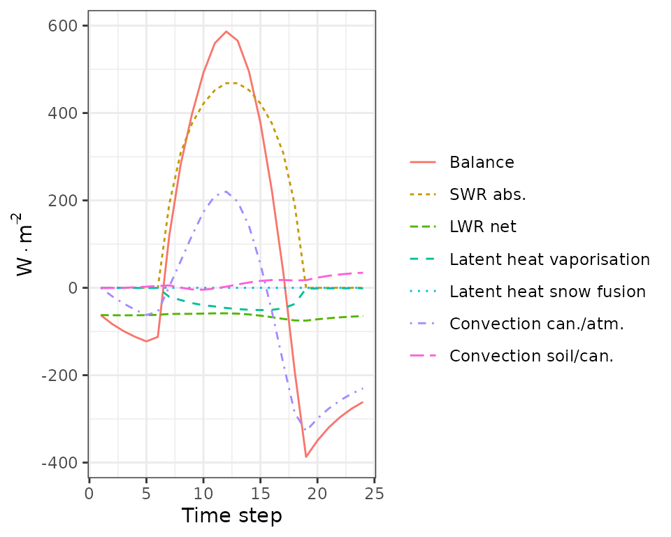

plot(sd1, type = "SoilEnergyBalance")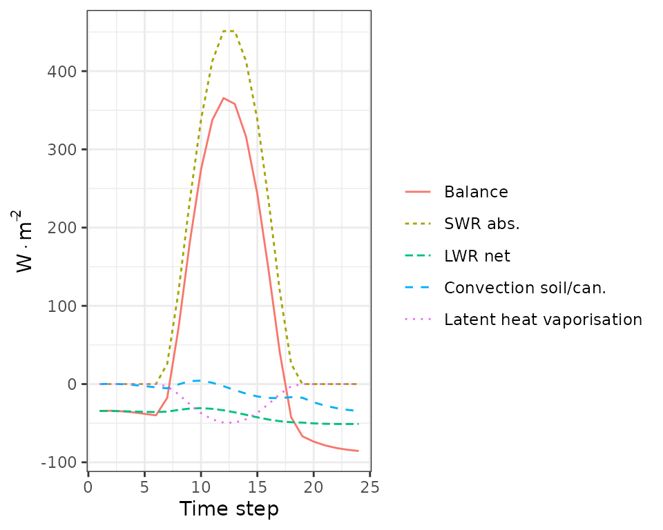

Plant output

Element Plants contains output values by plant cohort. Several output variables can be inspected in this element.

sd1$Plants

##               LAI    LAIlive     FPAR Extraction Transpiration
## T1_148 0.84874773 0.84874773 92.18285 0.17456211    0.17456211
## T2_168 0.70557382 0.70557382 72.36365 0.26548784    0.26548784
## S1_165 0.03062604 0.03062604 44.32407 0.01248587    0.01248587
##        GrossPhotosynthesis NetPhotosynthesis    RootPsi    StemPsi LeafPLC
## T1_148          1.93013613        1.81595972 -0.2180120 -0.6186918       0
## T2_168          1.79053535        1.68209560 -0.3785782 -0.9685505       0
## S1_165          0.06701287        0.06306827 -0.3759137 -0.6029081       0
##             StemPLC LeafPsiMin  LeafPsiMax      dEdP        DDS   StemRWC
## T1_148 0.0000155601 -0.8045533 -0.03995231 0.4783679 0.05133574 0.9987580
## T2_168 0.0097008380 -1.2294457 -0.04019149 0.5389841 0.03270465 0.9910449
## S1_165 0.0001971280 -0.7151737 -0.04188680 1.0414421 0.02823879 0.9879970
##          LeafRWC      LFMC  WaterBalance
## T1_148 0.9812122 124.74831 -1.051676e-17
## T2_168 0.9809096  91.79603  9.486769e-18
## S1_165 0.9890301  95.41927  1.162129e-18

While Plants contains one value per cohort and variable that summarizes the whole simulated day, information by disaggregated by time step can be accessed in PlantsInst. Moreover, we can use function plot.spwb_day() to draw plots of sub-daily variation per species of plant transpiration per ground area (L·m$^{-2}$), transpiration per leaf area (also in L·m$^{-2}$), plant net photosynthesis (in g C·m$^{-2}$), and plant water potential (in MPa):

plot(sd1, type = "PlantTranspiration", bySpecies = T)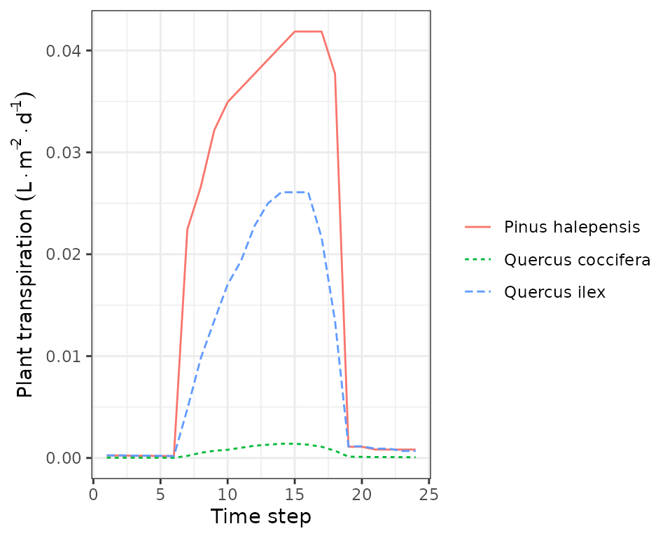

plot(sd1, type = "TranspirationPerLeaf", bySpecies = T)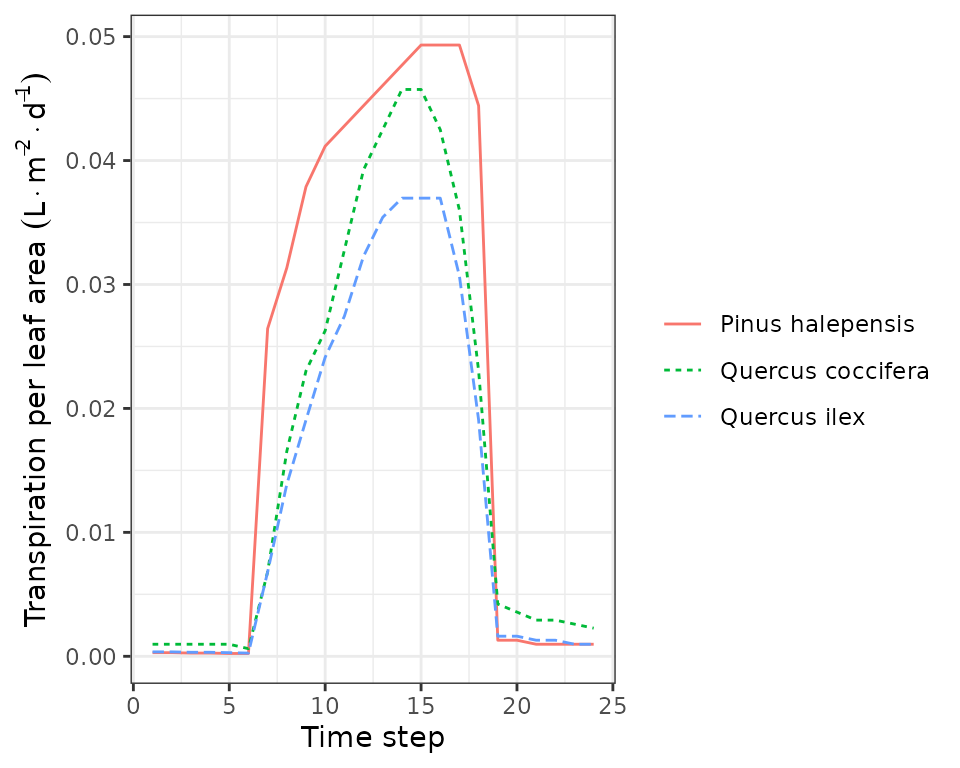

plot(sd1, type = "NetPhotosynthesis", bySpecies = T)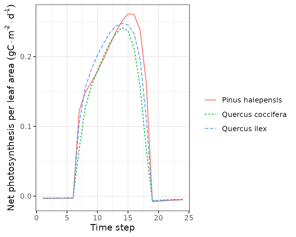

plot(sd1, type = "LeafPsiAverage", bySpecies = T)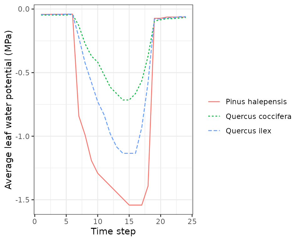

Output for sunlit and shade leaves

The model distinguishes between sunlit and shade leaves for stomatal regulation. Static properties of sunlit and shade leaves, for each cohort, can be accessed via:

sd1$SunlitLeaves

##        LeafPsiMin  LeafPsiMax      GSWMin     GSWMax  TempMin  TempMax
## T1_148 -0.9075917 -0.03995231 0.002274007 0.07232662 1.001841 12.35374
## T2_168 -1.6359558 -0.04198952 0.003269166 0.09304306 1.272433 17.63836
## S1_165 -1.1220604 -0.04703362 0.007561899 0.09612847 1.267823 17.42739

sd1$ShadeLeaves

##        LeafPsiMin  LeafPsiMax      GSWMin     GSWMax   TempMin  TempMax
## T1_148 -0.6506161 -0.03995231 0.002250501 0.06650165 0.9829446 10.50330
## T2_168 -0.8756072 -0.04019149 0.003263123 0.11879815 0.5326568 10.49146
## S1_165 -0.5152537 -0.04188680 0.007626981 0.10585774 0.6721882 10.29561

Instantaneous values are also stored for sunlit and shade leaves. We can also use the plot function for objects of class spwb_day to draw instantaneous variations in temperature for sunlit and shade leaves:

plot(sd1, type = "LeafTemperature", bySpecies=TRUE)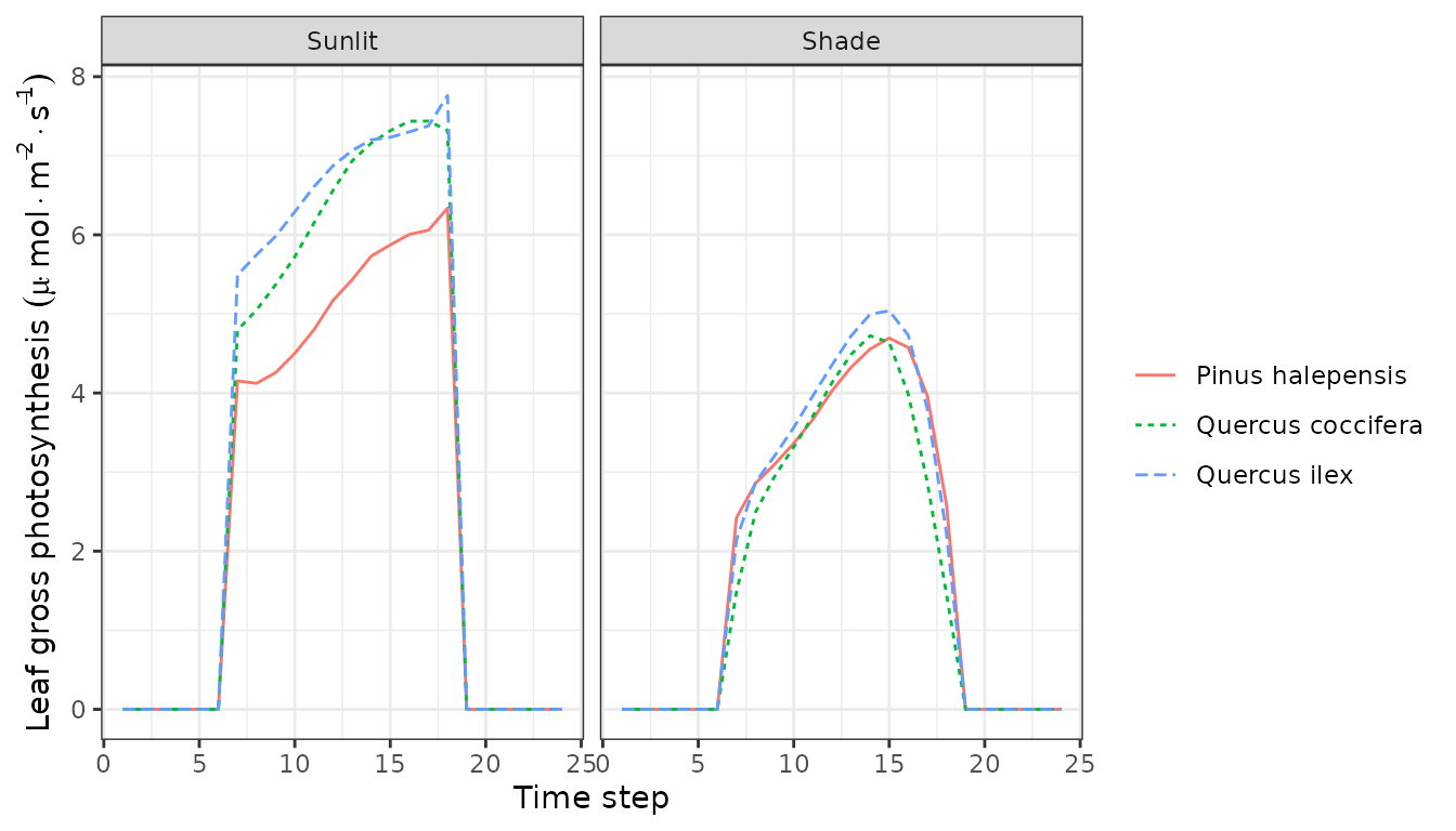

Note that sunlit leaves of some species reach temperatures higher than the canopy. We can also plot variations in instantaneous gross and net photosynthesis rates:

plot(sd1, type = "LeafGrossPhotosynthesis", bySpecies=TRUE)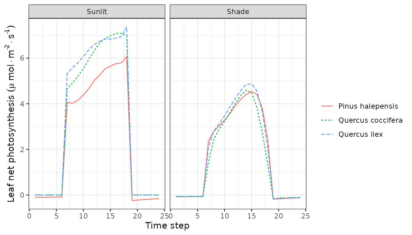

plot(sd1, type = "LeafNetPhotosynthesis", bySpecies=TRUE)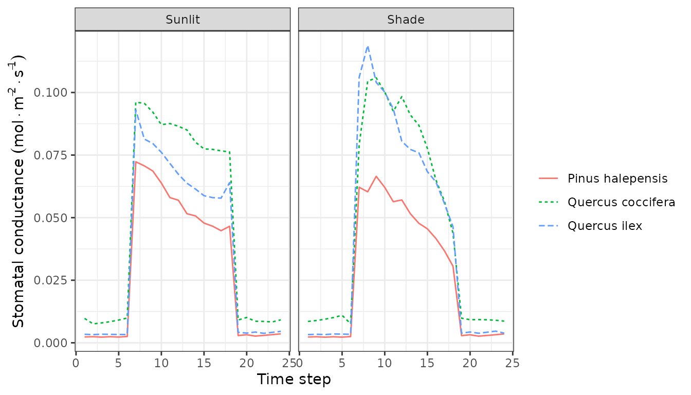

Or variations in stomatal conductance:

plot(sd1, type = "LeafStomatalConductance", bySpecies=TRUE)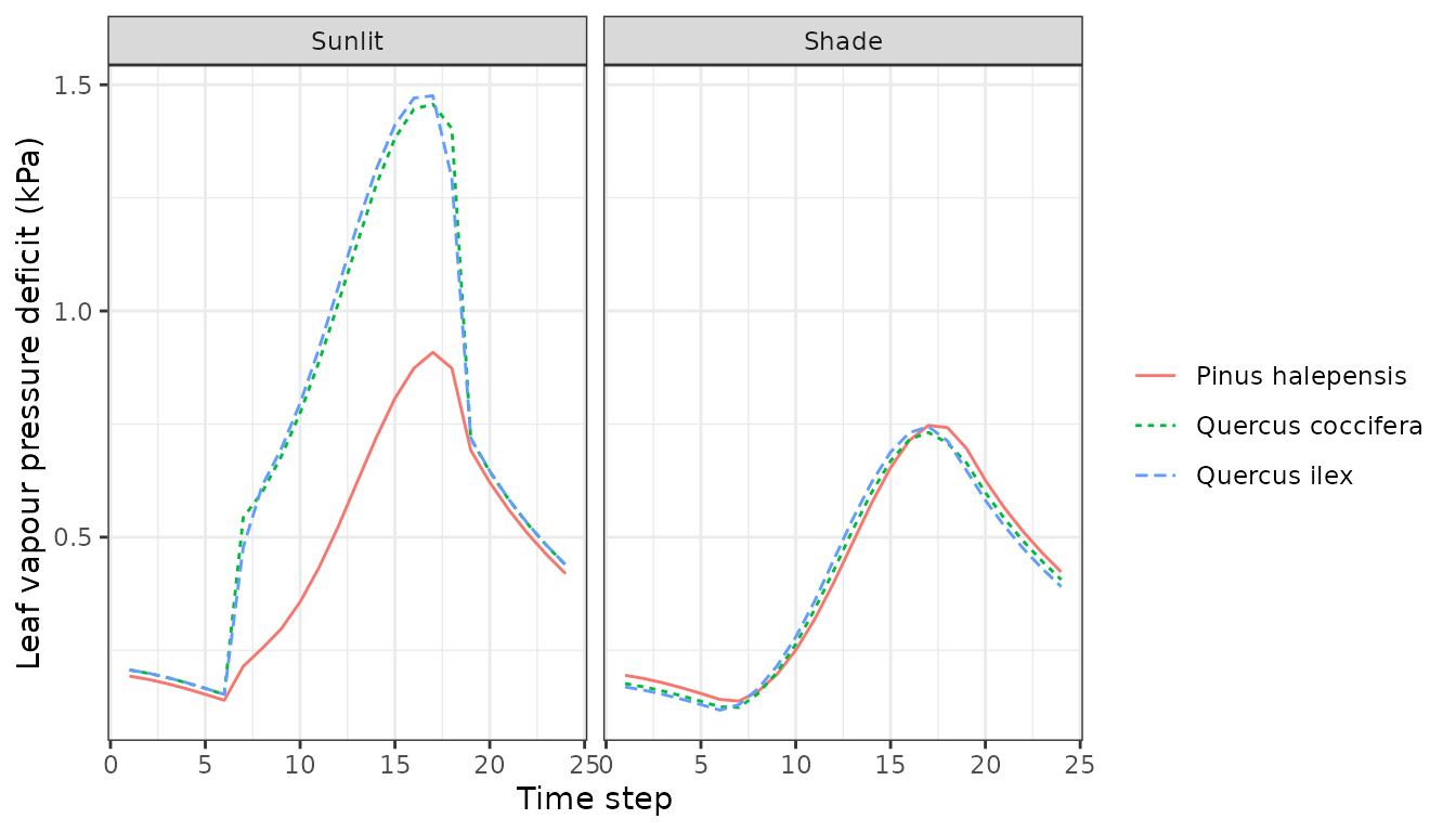

Or variations in vapour pressure deficit:

plot(sd1, type = "LeafVPD", bySpecies=TRUE)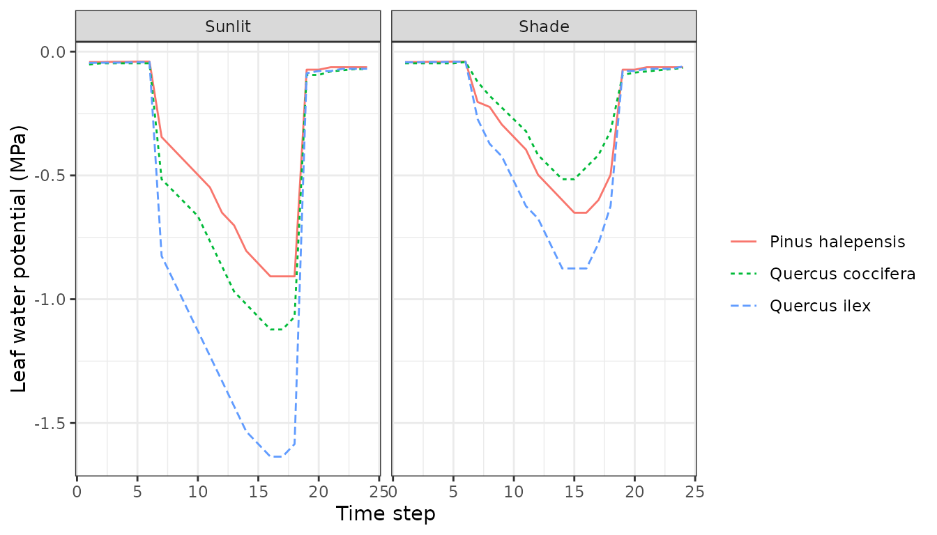

Or variations in leaf water potential:

plot(sd1, type = "LeafPsi", bySpecies=TRUE)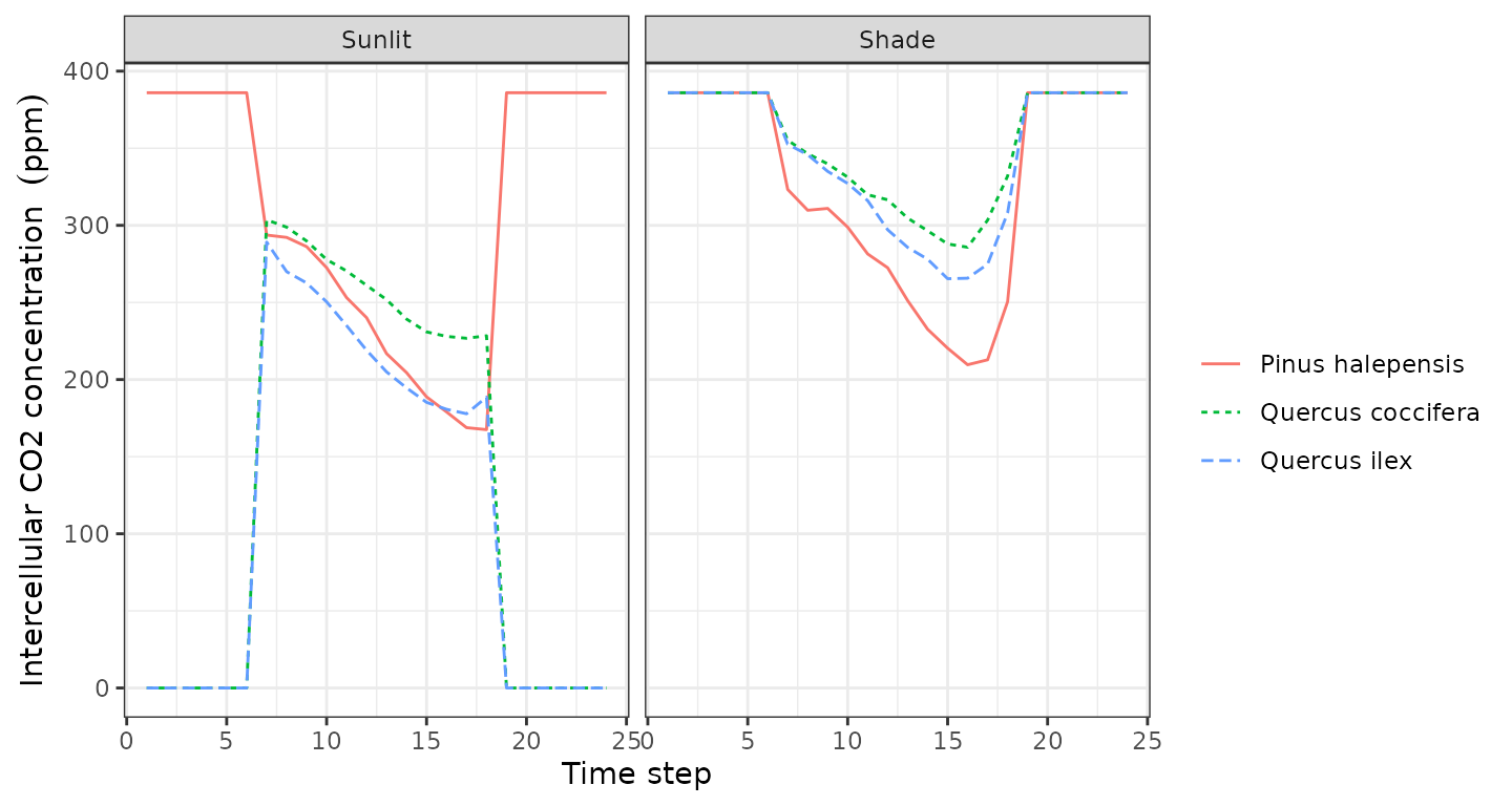

plot(sd1, type = "LeafCi", bySpecies=TRUE)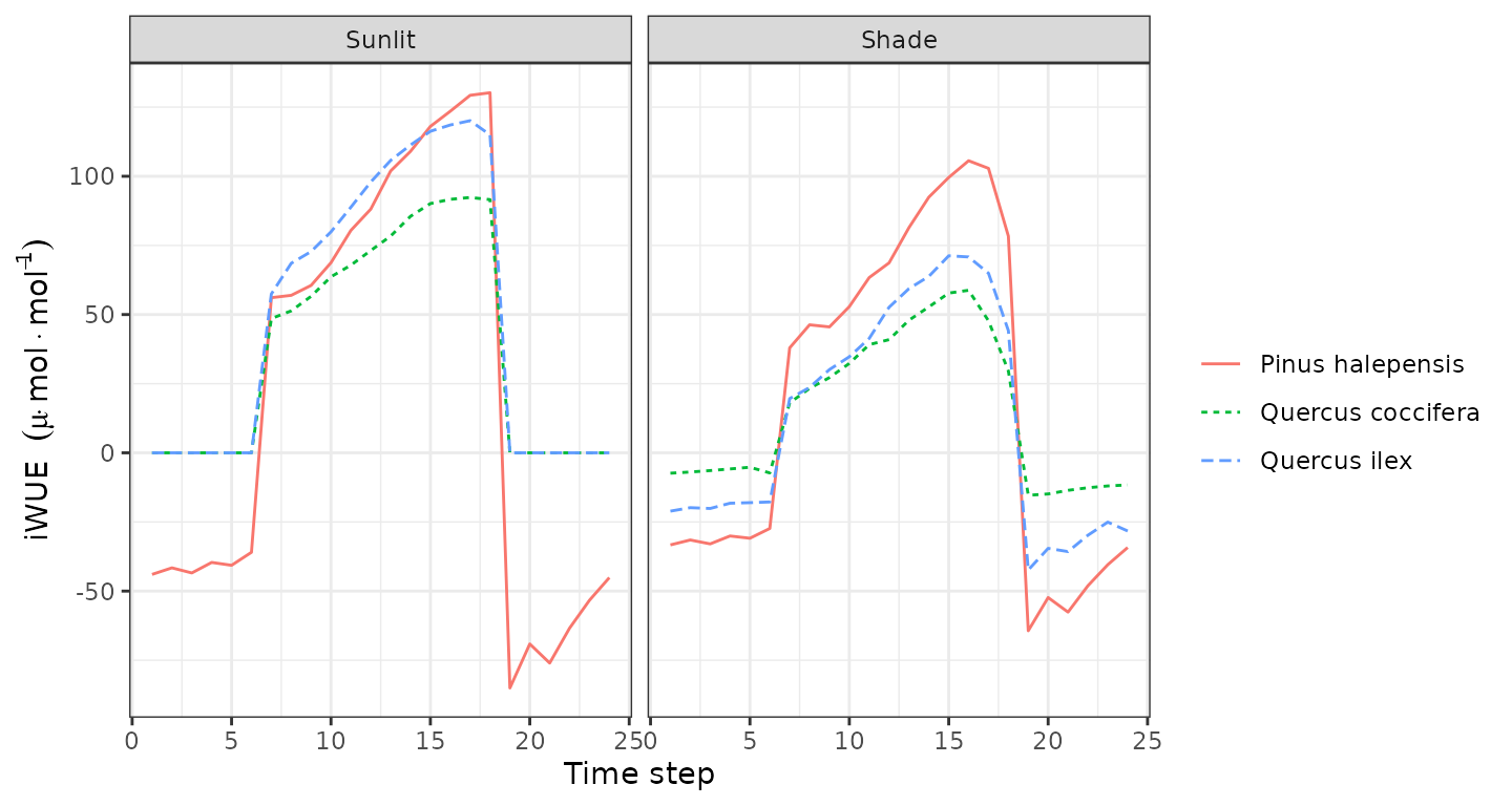

plot(sd1, type = "LeafIntrinsicWUE", bySpecies=TRUE)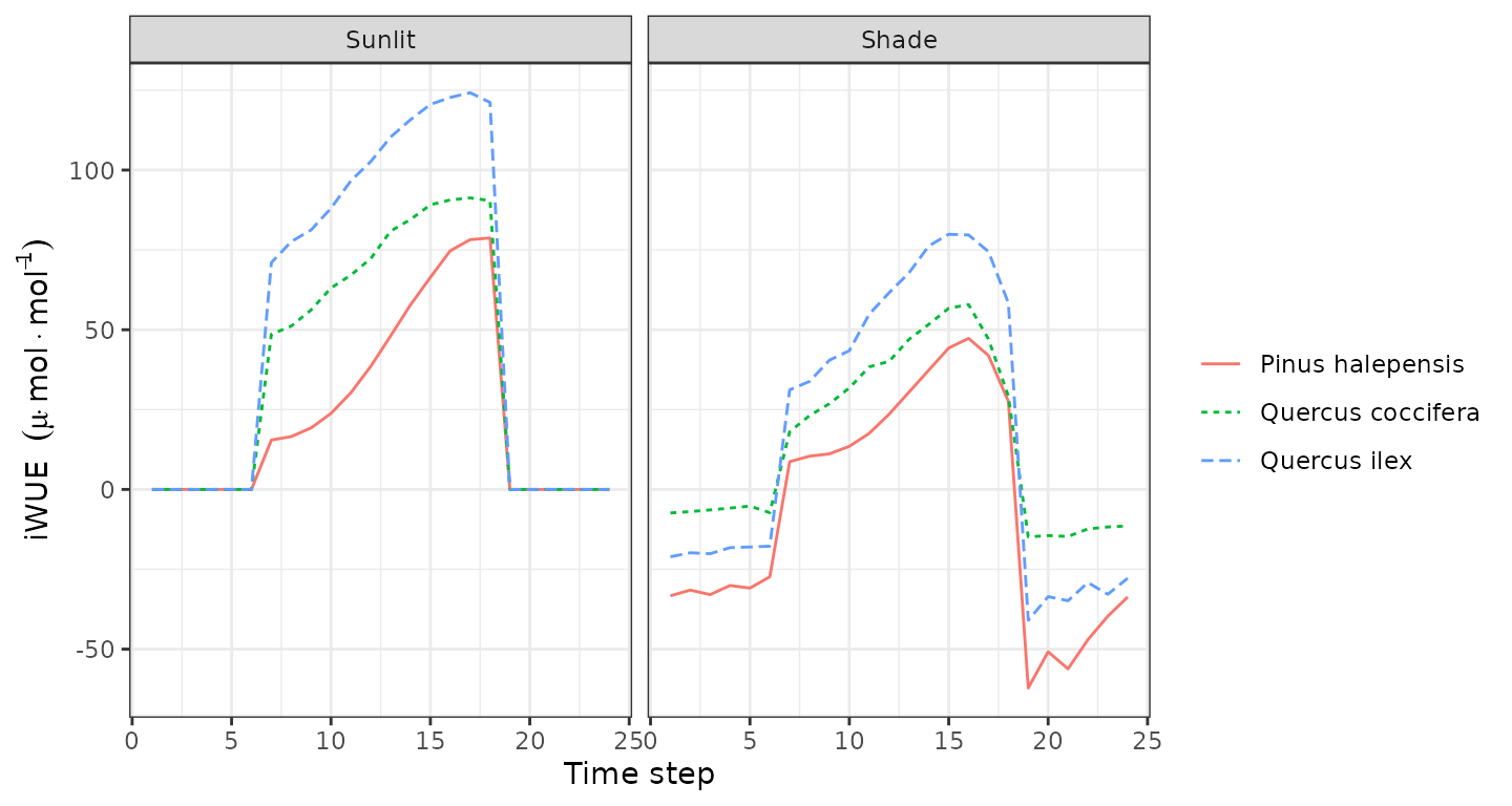

Water balance for multiple days

Running the model

Users will often use function spwb() to run the soil water balance model for several days. This function requires the spwbInput object, the soil object and the meteorological data frame. However, running spwb_day() modified the input objects. In particular, the soil moisture at the end of the simulation was:

x$soil$W

## [1] 0.9869450 0.9988968 1.0000958 1.0001638

And the temperature of soil layers:

x$soil$Temp

## [1] 8.157410 3.166508 2.383780 2.363290

We can also see the current state of canopy variables:

x$canopy

##    zlow zmid  zup     Tair Cair     VPair
## 1     0   50  100 5.735859  386 0.5170718
## 2   100  150  200 5.735859  386 0.5170718
## 3   200  250  300 5.735859  386 0.5170718
## 4   300  350  400 5.735859  386 0.5170718
## 5   400  450  500 5.735859  386 0.5170718
## 6   500  550  600 5.735859  386 0.5170718
## 7   600  650  700 5.735859  386 0.5170718
## 8   700  750  800 5.735859  386 0.5170718
## 9   800  850  900 5.735859  386 0.5170718
## 10  900  950 1000 5.735859  386 0.5170718
## 11 1000 1050 1100 5.735859  386 0.5170718
## 12 1100 1150 1200 5.735859  386 0.5170718
## 13 1200 1250 1300 5.735859  386 0.5170718
## 14 1300 1350 1400 5.735859  386 0.5170718
## 15 1400 1450 1500 5.735859  386 0.5170718
## 16 1500 1550 1600 5.735859  386 0.5170718
## 17 1600 1650 1700 5.735859  386 0.5170718
## 18 1700 1750 1800 5.735859  386 0.5170718
## 19 1800 1850 1900 5.735859  386 0.5170718
## 20 1900 1950 2000 5.735859  386 0.5170718
## 21 2000 2050 2100 5.735859  386 0.5170718
## 22 2100 2150 2200 5.735859  386 0.5170718
## 23 2200 2250 2300 5.735859  386 0.5170718
## 24 2300 2350 2400 5.735859  386 0.5170718
## 25 2400 2450 2500 5.735859  386 0.5170718
## 26 2500 2550 2600 5.735859  386 0.5170718
## 27 2600 2650 2700 5.735859  386 0.5170718
## 28 2700 2750 2800 5.735859  386 0.5170718

We simply use function resetInputs() to reset state variables to their default values, so that the new simulation is not affected by the end state of the previous simulation:

resetInputs(x)
x$soil$W

## [1] 1 1 1 1

x$soil$Temp

## [1] NA NA NA NA

x$canopy

##    zlow zmid  zup Tair Cair VPair
## 1     0   50  100   NA   NA    NA
## 2   100  150  200   NA   NA    NA
## 3   200  250  300   NA   NA    NA
## 4   300  350  400   NA   NA    NA
## 5   400  450  500   NA   NA    NA
## 6   500  550  600   NA   NA    NA
## 7   600  650  700   NA   NA    NA
## 8   700  750  800   NA   NA    NA
## 9   800  850  900   NA   NA    NA
## 10  900  950 1000   NA   NA    NA
## 11 1000 1050 1100   NA   NA    NA
## 12 1100 1150 1200   NA   NA    NA
## 13 1200 1250 1300   NA   NA    NA
## 14 1300 1350 1400   NA   NA    NA
## 15 1400 1450 1500   NA   NA    NA
## 16 1500 1550 1600   NA   NA    NA
## 17 1600 1650 1700   NA   NA    NA
## 18 1700 1750 1800   NA   NA    NA
## 19 1800 1850 1900   NA   NA    NA
## 20 1900 1950 2000   NA   NA    NA
## 21 2000 2050 2100   NA   NA    NA
## 22 2100 2150 2200   NA   NA    NA
## 23 2200 2250 2300   NA   NA    NA
## 24 2300 2350 2400   NA   NA    NA
## 25 2400 2450 2500   NA   NA    NA
## 26 2500 2550 2600   NA   NA    NA
## 27 2600 2650 2700   NA   NA    NA
## 28 2700 2750 2800   NA   NA    NA

Now we are ready to call function spwb():

S <- spwb(x, examplemeteo, latitude = 41.82592, elevation = 100)

## Initial plant water content (mm): 6.78662
## Initial soil water content (mm): 290.875
## Initial snowpack content (mm): 0
## Performing daily simulations
## 
##  [Year 2001]:....................................
## 
## Final plant water content (mm): 6.78287
## Final soil water content (mm): 342.354
## Final snowpack content (mm): 0
## Change in plant water content (mm): -0.00375222
## Plant water balance result (mm): -6.59433
## Change in soil water content (mm): 51.4795
## Soil water balance result (mm): 51.4795
## Change in snowpack water content (mm): 0
## Snowpack water balance result (mm): -7.10543e-15
## Water balance components:
##   Precipitation (mm) 513 Rain (mm) 462 Snow (mm) 51
##   Interception (mm) 92 Net rainfall (mm) 370
##   Infiltration (mm) 393 Infiltration excess (mm) 28 Saturation excess (mm) 0 Capillarity rise (mm) 3
##   Soil evaporation (mm) 11  Herbaceous transpiration (mm) 14 Woody plant transpiration (mm) 171
##   Plant extraction from soil (mm) 164  Plant water balance (mm) -7 Hydraulic redistribution (mm) 1
##   Runoff (mm) 28 Deep drainage (mm) 156

Function spwb() returns an object of class spwb. If we inspect its elements, we realize that the output is arranged differently than in spwb_day():

names(S)

##  [1] "latitude"      "topography"    "weather"       "spwbInput"    
##  [5] "spwbOutput"    "WaterBalance"  "EnergyBalance" "Temperature"  
##  [9] "Soil"          "Stand"         "Plants"        "SunlitLeaves" 
## [13] "ShadeLeaves"

In particular, element spwbInput contains a copy of the input parameters that were used to run the model:

names(S$spwbInput)

##  [1] "control"             "soil"                "canopy"             
##  [4] "herbLAI"             "herbLAImax"          "cohorts"            
##  [7] "above"               "below"               "belowLayers"        
## [10] "paramsPhenology"     "paramsAnatomy"       "paramsInterception" 
## [13] "paramsTranspiration" "paramsWaterStorage"  "internalPhenology"  
## [16] "internalWater"       "internalFCCS"

As before, WaterBalance contains water balance components, but in this case in form of a data frame with days in rows:

head(S$WaterBalance)

##                  PET Precipitation      Rain Snow    NetRain Snowmelt
## 2001-01-01 0.8828475      4.869109  4.869109    0  3.4241795        0
## 2001-01-02 1.6375337      2.498292  2.498292    0  1.0717469        0
## 2001-01-03 1.3017026      0.000000  0.000000    0  0.0000000        0
## 2001-01-04 0.5690790      5.796973  5.796973    0  4.3625616        0
## 2001-01-05 1.6760567      1.884401  1.884401    0  0.7539027        0
## 2001-01-06 1.2077028     13.359801 13.359801    0 11.7240275        0
##            Infiltration InfiltrationExcess SaturationExcess Runoff DeepDrainage
## 2001-01-01    3.4241795                  0                0      0  0.005025398
## 2001-01-02    1.0717469                  0                0      0  0.005054727
## 2001-01-03    0.0000000                  0                0      0  0.005113967
## 2001-01-04    4.3625616                  0                0      0  0.005115942
## 2001-01-05    0.7539027                  0                0      0  0.005149149
## 2001-01-06   11.7240275                  0                0      0  0.005182355
##            CapillarityRise Evapotranspiration Interception SoilEvaporation
## 2001-01-01    4.745735e-05          1.9081746     1.444929      0.44789475
## 2001-01-02    4.145186e-05          1.5393365     1.426545      0.06352600
## 2001-01-03    0.000000e+00          0.2671073     0.000000      0.04897017
## 2001-01-04    4.089020e-04          1.5026996     1.434411      0.05535087
## 2001-01-05    4.085636e-05          1.2386952     1.130499      0.02403944
## 2001-01-06    5.035626e-03          1.6760275     1.635773      0.02271906
##            HerbTranspiration PlantExtraction Transpiration
## 2001-01-01       0.011023432     0.004327076   0.004327076
## 2001-01-02       0.020448234     0.009692228   0.028817522
## 2001-01-03       0.016254970     0.201882116   0.201882116
## 2001-01-04       0.007106285     0.005831135   0.005831135
## 2001-01-05       0.020931252     0.023303572   0.063225764
## 2001-01-06       0.015082370     0.002452908   0.002452908
##            HydraulicRedistribution
## 2001-01-01            0.000000e+00
## 2001-01-02            2.162440e-05
## 2001-01-03            2.077891e-05
## 2001-01-04            6.512726e-05
## 2001-01-05            2.512755e-03
## 2001-01-06            3.063577e-03

Elements Plants is itself a list with several elements that contain daily output results by plant cohorts, for example leaf minimum (midday) water potentials are:

head(S$Plants$LeafPsiMin)

##                T1_148     T2_168     S1_165
## 2001-01-01 -0.4112408 -0.7886543 -0.3902716
## 2001-01-02 -0.4710891 -0.7468420 -0.3926637
## 2001-01-03 -0.5344002 -0.9090484 -0.4988152
## 2001-01-04 -0.3725677 -0.6995837 -0.3434085
## 2001-01-05 -0.4965693 -0.8256897 -0.4237924
## 2001-01-06 -0.4456530 -0.7249563 -0.3739271

Plotting and summarizing results

Package medfate also provides a plot function for objects of class spwb. It can be used to show the meteorological input. Additionally, it can also be used to draw soil and plant variables. In the code below we draw water fluxes, soil water potentials, plant transpiration and plant (mid-day) water potential:

plot(S, type="Evapotranspiration")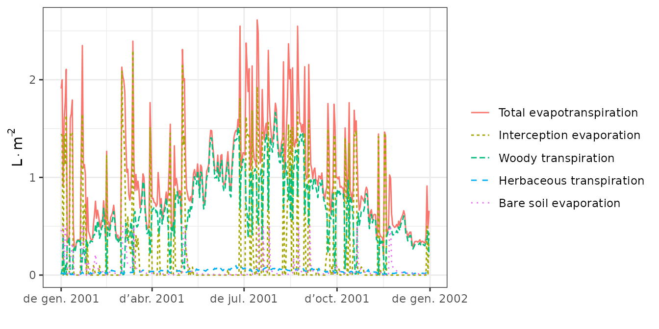

plot(S, type="SoilPsi", bySpecies = TRUE)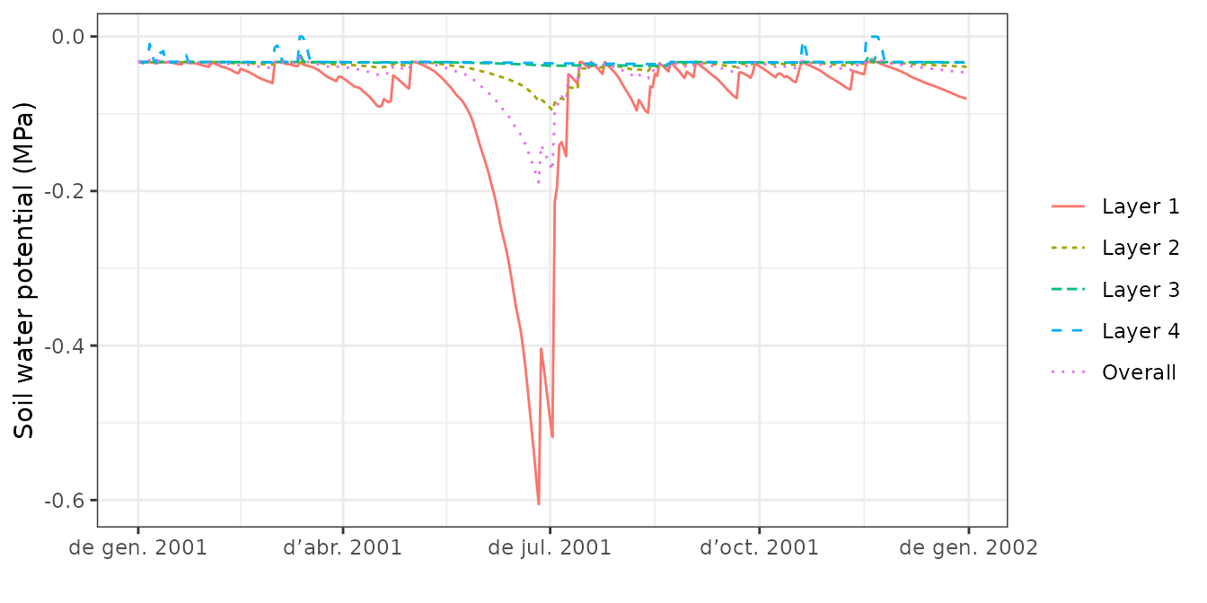

plot(S, type="PlantTranspiration", bySpecies = TRUE)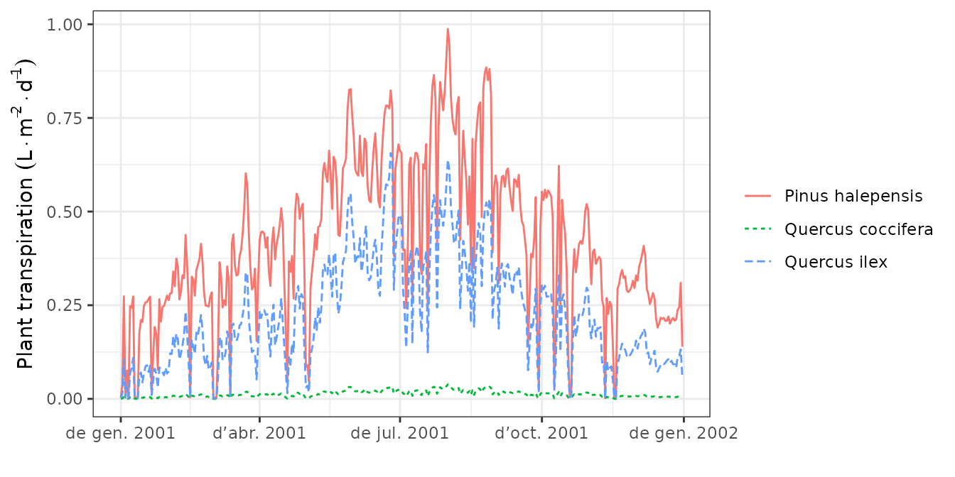

plot(S, type="LeafPsiMin", bySpecies = TRUE)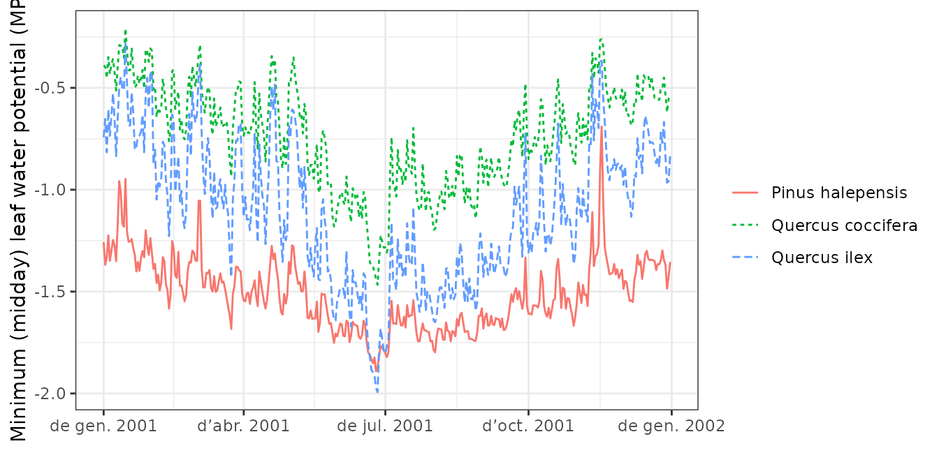

Alternatively, one can interactively create plots using function shinyplot, e.g.:

shinyplot(S)

While the simulation model uses daily steps, users may be interested in outputs at larger time scales. The package provides a summary for objects of class spwb. This function can be used to summarize the model’s output at different temporal steps (i.e. weekly, annual, …). For example, to obtain the average soil moisture and water potentials by months one can use:

summary(S, freq="months",FUN=mean, output="Soil")

##                  W.1      W.2      W.3      W.4     ML.1     ML.2      ML.3
## 2001-01-01 1.1878032 1.137118 1.043172 1.012412 80.97707 132.6482  79.01888
## 2001-02-01 1.1261697 1.196878 1.200532 1.120964 76.77528 139.6193  90.93872
## 2001-03-01 1.1904179 1.258730 1.322533 1.354367 81.15533 146.8346 100.18016
## 2001-04-01 1.0474333 1.170981 1.282016 1.388142 71.40752 136.5984  97.11100
## 2001-05-01 1.0656435 1.159531 1.248185 1.369492 72.64898 135.2627  94.54837
## 2001-06-01 0.8052586 1.042451 1.193040 1.345024 54.89755 121.6050  90.37117
## 2001-07-01 1.0576171 1.086765 1.159710 1.313601 72.10179 126.7744  87.84652
## 2001-08-01 1.0795432 1.147316 1.207276 1.341697 73.59657 133.8379  91.44960
## 2001-09-01 1.0859284 1.163617 1.242915 1.370995 74.03188 135.7394  94.14914
## 2001-10-01 1.1099954 1.162690 1.236029 1.365037 75.67262 135.6312  93.62754
## 2001-11-01 1.1622470 1.220831 1.277275 1.377036 79.23481 142.4135  96.75193
## 2001-12-01 1.0821919 1.208661 1.293211 1.384088 73.77715 140.9939  97.95902
##                ML.4    MLTot SaturatedDepth        SWE PlantExt.1 PlantExt.2
## 2001-01-01 30.67555 323.3197      3412.3362 1.65619239 0.07274422 0.03182156
## 2001-02-01 33.96463 341.2980      2412.2259 0.27608905 0.17958576 0.09394033
## 2001-03-01 41.03660 369.2067       774.4905 0.01762496 0.17533687 0.09128468
## 2001-04-01 42.05997 347.1768      1025.3574 0.58072652 0.24042132 0.13149380
## 2001-05-01 41.49490 343.9550      1190.1897 0.00000000 0.36707238 0.19483588
## 2001-06-01 40.75351 307.6273      1725.7818 0.00000000 0.48671847 0.34286476
## 2001-07-01 39.80141 326.5241      1775.6024 0.00000000 0.44713446 0.23431546
## 2001-08-01 40.65272 339.5368      1430.5119 0.00000000 0.50487865 0.25326115
## 2001-09-01 41.54044 345.4609      1175.5734 0.00000000 0.32752264 0.16819212
## 2001-10-01 41.35990 346.2913      1204.3111 0.00000000 0.26895826 0.13599375
## 2001-11-01 41.72345 360.1237       880.7175 2.60802857 0.15605882 0.08227887
## 2001-12-01 41.93715 354.6672       938.2599 0.00000000 0.14230673 0.08141877
##             PlantExt.3   PlantExt.4 HydraulicInput.1 HydraulicInput.2
## 2001-01-01 0.001828883 0.0003328499     0.000000e+00     8.748800e-04
## 2001-02-01 0.007589478 0.0009646686     4.183673e-05     0.000000e+00
## 2001-03-01 0.007459551 0.0026991194     2.864977e-04     5.840216e-05
## 2001-04-01 0.011299189 0.0016039369     8.403879e-04     0.000000e+00
## 2001-05-01 0.016470375 0.0022513480     4.222118e-04     0.000000e+00
## 2001-06-01 0.029848632 0.0039962718     1.019459e-02     0.000000e+00
## 2001-07-01 0.019828490 0.0027715571     3.561568e-03     1.796264e-05
## 2001-08-01 0.021043509 0.0028821835     7.014275e-05     0.000000e+00
## 2001-09-01 0.014202750 0.0019712019     2.822305e-04     0.000000e+00
## 2001-10-01 0.011571473 0.0016777922     1.172672e-04     5.043713e-06
## 2001-11-01 0.006960953 0.0018480398     2.056153e-04     6.161136e-05
## 2001-12-01 0.006987310 0.0011257329     1.201171e-04     0.000000e+00
##            HydraulicInput.3 HydraulicInput.4       psi.1       psi.2
## 2001-01-01     4.511995e-04     7.363076e-05 -0.01305674 -0.01737078
## 2001-02-01     2.372451e-06     1.298834e-05 -0.01870026 -0.01232861
## 2001-03-01     2.179680e-06     0.000000e+00 -0.01316292 -0.00809235
## 2001-04-01     0.000000e+00     0.000000e+00 -0.02691589 -0.01431356
## 2001-05-01     0.000000e+00     0.000000e+00 -0.02685265 -0.01523164
## 2001-06-01     0.000000e+00     0.000000e+00 -0.09330172 -0.02777884
## 2001-07-01     0.000000e+00     0.000000e+00 -0.03237115 -0.02213668
## 2001-08-01     0.000000e+00     0.000000e+00 -0.02367656 -0.01603404
## 2001-09-01     0.000000e+00     0.000000e+00 -0.02235840 -0.01473428
## 2001-10-01     0.000000e+00     0.000000e+00 -0.02016726 -0.01475783
## 2001-11-01     1.560947e-06     0.000000e+00 -0.01594455 -0.01070379
## 2001-12-01     0.000000e+00     0.000000e+00 -0.02294043 -0.01158654
##                   psi.3         psi.4
## 2001-01-01 -0.026799332 -0.0309657171
## 2001-02-01 -0.011732308 -0.0183039792
## 2001-03-01 -0.004374725 -0.0023024420
## 2001-04-01 -0.006940588 -0.0008059514
## 2001-05-01 -0.008779147 -0.0019955323
## 2001-06-01 -0.012632697 -0.0033789854
## 2001-07-01 -0.014901647 -0.0049903423
## 2001-08-01 -0.011323421 -0.0034119389
## 2001-09-01 -0.009064340 -0.0018926725
## 2001-10-01 -0.009468937 -0.0022237858
## 2001-11-01 -0.006902060 -0.0014213876
## 2001-12-01 -0.006411571 -0.0010907396

Parameter output is used to indicate the element of the spwb object for which we desire summaries. Similarly, it is possible to calculate the average stress of plant cohorts by months:

summary(S, freq="months",FUN=mean, output="PlantStress")

##                T1_148     T2_168      S1_165
## 2001-01-01 0.01681590 0.01131279 0.008694034
## 2001-02-01 0.03193405 0.02285562 0.016003470
## 2001-03-01 0.03650643 0.02652692 0.018229593
## 2001-04-01 0.04489949 0.03294030 0.023697445
## 2001-05-01 0.06482891 0.04748175 0.034931760
## 2001-06-01 0.11462159 0.07718295 0.064082996
## 2001-07-01 0.09344463 0.06689288 0.049204666
## 2001-08-01 0.09329027 0.06884827 0.049623986
## 2001-09-01 0.06202276 0.04645234 0.032186031
## 2001-10-01 0.05039116 0.03677347 0.024769483
## 2001-11-01 0.02638692 0.02010258 0.013279552
## 2001-12-01 0.02613260 0.01859706 0.013638821

The summary function can be also used to aggregate the output by species. In this case, the values of plant cohorts belonging to the same species will be averaged using LAI values as weights. For example, we may average the daily drought stress across cohorts of the same species (here there is only one cohort by species, so this does not modify the output):

head(summary(S, freq="day", output="PlantStress", bySpecies = TRUE))

##            Pinus halepensis Quercus coccifera Quercus ilex
## 2001-01-01       0.01587626       0.009798356   0.01121120
## 2001-01-02       0.01779665       0.009427698   0.01179912
## 2001-01-03       0.02040035       0.013083981   0.01549564
## 2001-01-04       0.01444006       0.008631081   0.01212184
## 2001-01-05       0.01729515       0.009201020   0.01210149
## 2001-01-06       0.01395796       0.007587623   0.01038485

Or we can combine the aggregation by species with a temporal aggregation (here monthly averages):

summary(S, freq="month", FUN = mean, output="PlantStress", bySpecies = TRUE)

##            Pinus halepensis Quercus coccifera Quercus ilex
## 2001-01-01       0.01681590       0.008694034   0.01131279
## 2001-02-01       0.03193405       0.016003470   0.02285562
## 2001-03-01       0.03650643       0.018229593   0.02652692
## 2001-04-01       0.04489949       0.023697445   0.03294030
## 2001-05-01       0.06482891       0.034931760   0.04748175
## 2001-06-01       0.11462159       0.064082996   0.07718295
## 2001-07-01       0.09344463       0.049204666   0.06689288
## 2001-08-01       0.09329027       0.049623986   0.06884827
## 2001-09-01       0.06202276       0.032186031   0.04645234
## 2001-10-01       0.05039116       0.024769483   0.03677347
## 2001-11-01       0.02638692       0.013279552   0.02010258
## 2001-12-01       0.02613260       0.013638821   0.01859706

References

De Cáceres M, Mencuccini M, Martin-StPaul N, Limousin JM, Coll L, Poyatos R, Cabon A, Granda V, Forner A, Valladares F, Martínez-Vilalta J (2021) Unravelling the effect of species mixing on water use and drought stress in holm oak forests: a modelling approach. Agricultural and Forest Meteorology 296 (https://doi.org/10.1016/j.agrformet.2020.108233).
Ruffault J, Pimont F, Cochard H, Dupuy JL, Martin-StPaul N (2022) SurEau-Ecos v2.0: a trait-based plant hydraulics model for simulations of plant water status and drought-induced mortality at the ecosystem level. Geoscientific Model Development 15, 5593-5626 (https://doi.org/10.5194/gmd-15-5593-2022).

Miquel De Caceres

2024-04-16

About this vignette

Preparing model inputs

Soil, vegetation, meteorology and species data

Simulation control

Water balance input object

Static analysis of sub-models

Vulnerability curves

Supply functions

Stomatal regulation and photosynthesis

Pressure volume curves

Water balance for a single day

Running the model

Water balance output

Soil and canopy energy balance

Plant output

Output for sunlit and shade leaves

Water balance for multiple days

Running the model

Plotting and summarizing results

References