Calibration of growth and senescence parameters

Introduction

Goals

The growth model included in medfate implements processes regulating plant carbon balance and growth. Species-level parameter values for these processes are obtained from: (a) global functional trait databases; (b) meta-modelling exercises; (c) model calibration exercises. The main goal of the current exercise is to obtain suitable values (via model calibration) for parameters related with the maintenance respiration costs, formation rates and senescence rates of sapwood, because these are difficult to obtain using other means. At the same time, the exercise provides information on the performance of the model to predict secondary growth at the tree and stand levels.

The results presented here were obtained using ver. 4.7.0 of medfate.

Observational data

The calibration data set corresponds to 75 permanent forest plots of the Spanish National Forest Inventory located in Catalonia. Forest plots correspond to pure stands whose dominant species are Fagus sylvatica, Pinus halepensis, Pinus nigra, Pinus sylvestris or Quercus pubescens. There are 15 plots per each dominant species and each set of 15 plots encompass a range of climatic aridity. Plot characteristics are described in Rosas et al. (2019). Dendrochronological series are available for up to 6 trees per plot and were sampled in December 2015. Note that a sixth species (Quercus ilex) was included in Rosas et al (2019), but dendrochronological dating is not available.

Target parameters for calibration

The model parameters for which we desired good estimates are:

Sapwood daily respiration rate (RERsapwood) - Used to modulate maintenance respiration demands of living sapwood tissues (parenchyma, cambium, phloem, etc.), which in large trees may also represent a large fraction of maintenance respiration.
Sapwood maximum growth rate (RGRcambiummax) - Used to modulate tree maximum daily sapwood growth rates (relative to current cambium perimeter). Actual relative growth rates include temperature and sink limitations to growth.
Sapwood daily senescence rate (SRsapwood) - Used to determine the daily proportion of sapwood that becomes heartwood. It regulates the area of functional sapwood, together with the sapwood maximum growth rate.

In addition, soil stoniness in the target plots had been estimated from surface stoniness classes. Since soil rock fragment content (rfc) has a strong influence on soil water capacity, we decided to include the proportion of rocks in the second soil layer (between 30 and 100 cm) as a parameter to be calibrated.

Calibration procedure

For each forest plot in the first data set, we matched each available dendrochronological series with a forest inventory tree cohort by finding which tree (in the IFN3 sampling) had the DBH most similar to that estimated from the dendrochronology at year 2000. Then, we took the series of annual basal area increments (BAI) as the observations to be matched by model secondary growth predictions for the matched tree cohort. For each forest plot of the second data set, we took all available dendrochronological series between 1990 and 2004. Available diameter increments (DI) were used to infer DBH at year 1990 and we transformed DI into annual BAI.

Simulations were performed using daily weather data for each target plot, obtained via interpolation using package meteoland (2001 - 2015 period or 1990-2004 period, depending on the data set), and soil physical characteristics where drawn from SoilGrids data base. Model simulations were done using the basic water balance model (i.e. transpirationMode = "Granier"), which explains why evaluation of calibrated growth is better for this model than the advanced ones (i.e. Sperry or Sureau). Transpiration and photosynthesis parameters were given values resulting from the meta-modelling exercise, whereas other parameters of the sensitivity analysis were left to the species-level defaults of SpParamsMED. We calibrated the four target parameters for the target dominant species of the target plot using a genetic algorithm (function ga from package GA). Model parameter values were assumed to be the same for all cohorts of the target species, while the remaining species in the plot were given default constant parameter values. The objective function for the genetic algorithm was the average, across cohorts with observed dendrochronology series, of the mean absolute error (MAE) resulting from comparing observed and predicted annual BAI series. Population size for the genetic algorithm was set to 40 individuals. A maximum of 25 iterations of the genetic algorithm were allowed, and the calibration procedure stopped if the best parameter combination did not change during 5 consecutive iterations.

The following table shows the range of values explored for each parameter to be calibrated:

	Minimum	Maximum
RERsapwood	1.0e-06	1.0e-04
RGRcambiummax	1.0e-04	2.0e-02
SRsapwood	1.0e-05	2.5e-04
rfc@2	2.5e+01	9.5e+01

Calibration results

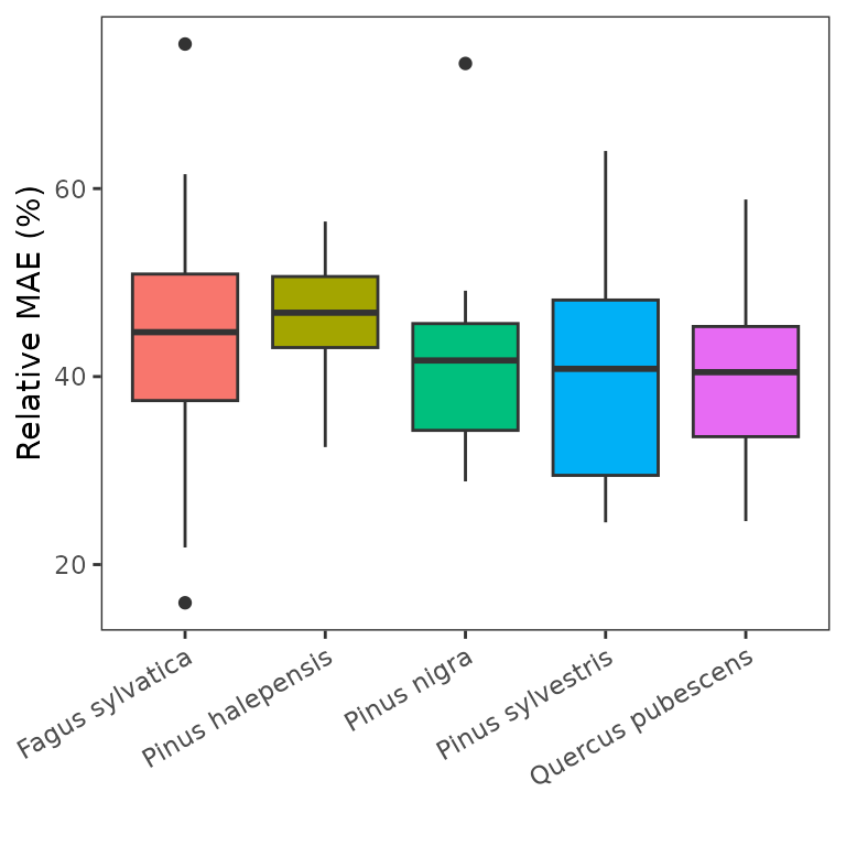
Error function

The following panel shows the distribution of the final (optimum) values of the error function (average relative MAE) by dominant species:

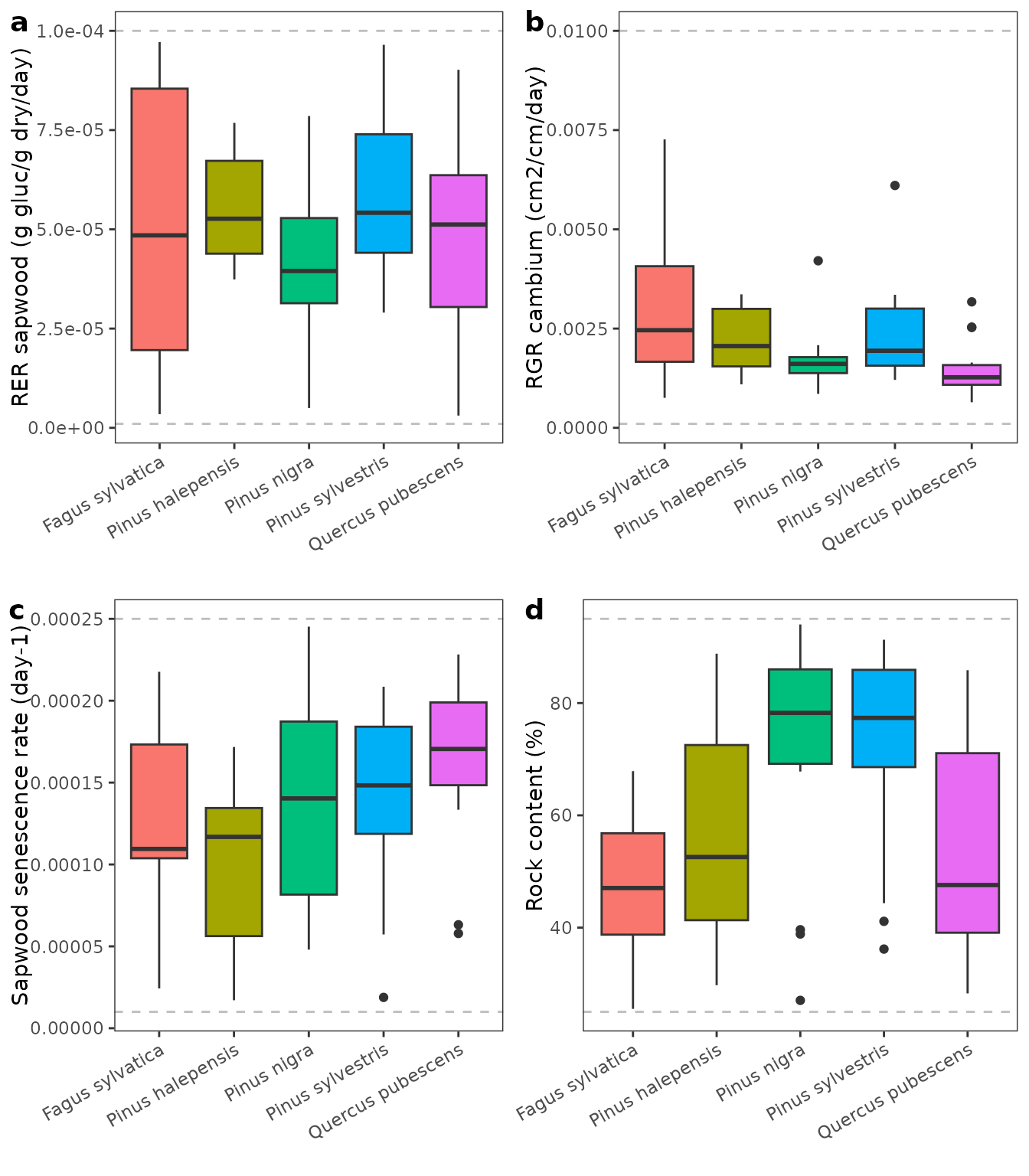
Parameter distribution and covariance

The following panels show the distribution of calibrated parameter values by species (gray dashed lines indicate the parameter value limits used in the calibration procedure):

The following table shows mean error and parameter values by species and overall means:

	value_cal	RERsapwood_cal	RGRcambiummax_cal	SRsapwood_cal	rfc_cal
Fagus sylvatica	44.58113	5.16e-05	0.0030927	0.0001391	67.64601
Pinus halepensis	50.12844	3.76e-05	0.0012879	0.0001432	72.04303
Pinus nigra	41.60647	5.45e-05	0.0013369	0.0001019	68.78204
Pinus sylvestris	46.40091	5.44e-05	0.0020224	0.0001305	65.11412
Quercus pubescens	38.80396	5.11e-05	0.0014198	0.0001173	61.55416
All	44.30418	4.98e-05	0.0018319	0.0001264	67.02787

Statistically significant differences can be observed between species for RERsapwood and RGRcambiummax, as shown in the following ANOVA tables:

## Analysis of Variance Table
## 
## Response: RERsapwood_cal
##           Df     Sum Sq    Mean Sq F value  Pr(>F)  
## Species    4 2.9387e-09 7.3468e-10  2.4538 0.05371 .
## Residuals 70 2.0958e-08 2.9941e-10                  
## ---
## Signif. codes:  0 '***' 0.001 '**' 0.01 '*' 0.05 '.' 0.1 ' ' 1

## Analysis of Variance Table
## 
## Response: RGRcambiummax_cal
##           Df     Sum Sq    Mean Sq F value    Pr(>F)    
## Species    4 3.5051e-05 8.7627e-06  7.2156 6.342e-05 ***
## Residuals 70 8.5008e-05 1.2144e-06                      
## ---
## Signif. codes:  0 '***' 0.001 '**' 0.01 '*' 0.05 '.' 0.1 ' ' 1

## Analysis of Variance Table
## 
## Response: SRsapwood_cal
##           Df     Sum Sq    Mean Sq F value  Pr(>F)  
## Species    4 1.7168e-08 4.2920e-09  2.6302 0.04147 *
## Residuals 70 1.1422e-07 1.6318e-09                  
## ---
## Signif. codes:  0 '***' 0.001 '**' 0.01 '*' 0.05 '.' 0.1 ' ' 1

## Analysis of Variance Table
## 
## Response: rfc_cal
##           Df  Sum Sq Mean Sq F value Pr(>F)
## Species    4   933.5  233.38  0.5634   0.69
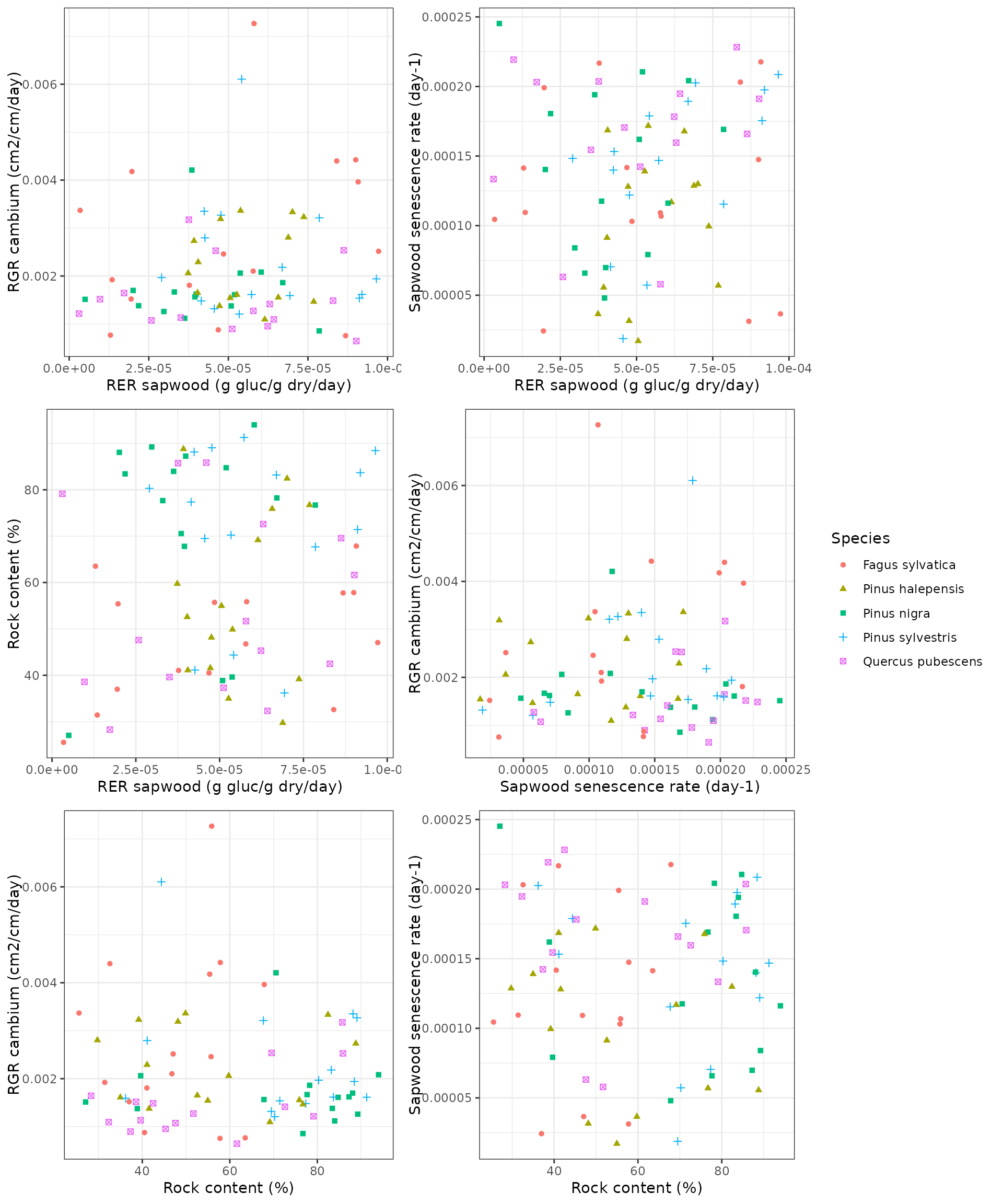
## Residuals 70 28996.7  414.24

Finally, the following panels illustrate the overall lack of covariance between calibrated parameter values:

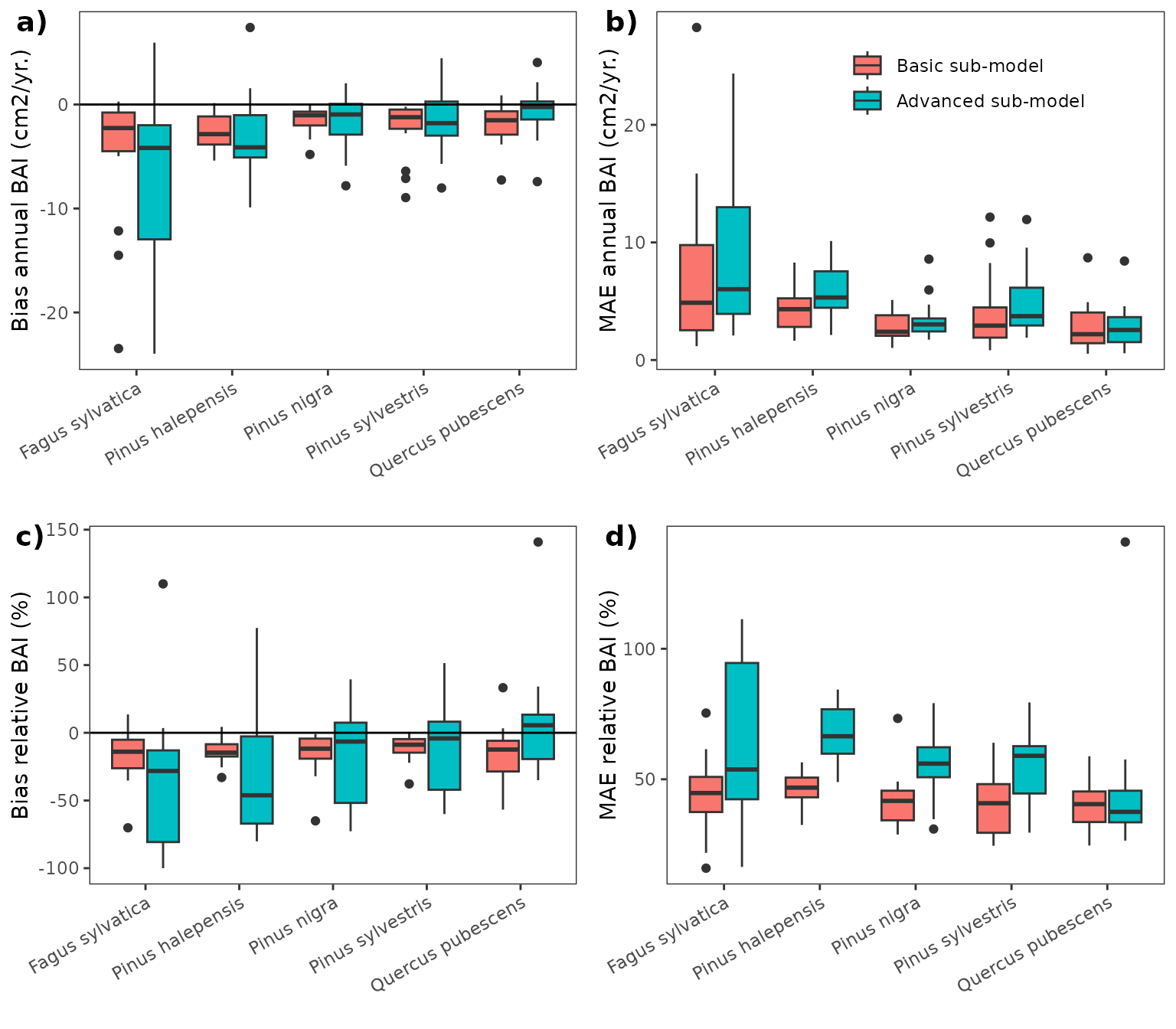
## Warning in get_plot_component(plot, "guide-box"): Multiple components found;
## returning the first one. To return all, use `return_all = TRUE`.

Comparison of the basic and advanced sub-models

Since the calibration exercise had been conducted using the basic sub-model (transpirationMode = "Granier"), it is expected that growth simulations with the advanced sub-model (transpirationMode = "Sperry" or transpirationMode = "Sureau") have larger error rates and, potentially, larger bias. To check this, we repeated growth simulations using the calibrated parameters for each plot and the advanced sub-model.

The following figures show the bias and mean absolute error of annual basal area increments obtained in simulations using the basic and advanced sub-models, in both cases using the calibrated parameters.

Bibliography

Batllori, E., J. M. Blanco-Moreno, J. M. Ninot, E. Gutiérrez, and E. Carrillo. 2009. Vegetation patterns at the alpine treeline ecotone: the influence of tree cover on abrupt change in species composition of alpine communities. Journal of Vegetation Science 20:814–825.
Batllori, E., and E. Gutiérrez. 2008. Regional tree line dynamics in response to global change in the Pyrenees. Journal of Ecology 96:1275–1288.
Rosas, T., M. Mencuccini, J. Barba, H. Cochard, S. Saura-Mas, and J. Martínez-Vilalta. 2019. Adjustments and coordination of hydraulic, leaf and stem traits along a water availability gradient. New Phytologist 223:632–646.

Miquel De Cáceres

2024-11-05