Chapter 3 Basic water balance model
This chapter provides an overview of the basic soil and plant water balance model included in medfate. The model allows simulating vertical water fluxes in a forest stand, and performs soil and plant water balance on a daily step basis for the period corresponding to input weather data.
The model is run using function spwb(), for a set of days, or function spwb_day(), for a single day. The basic water balance model corresponds to the control variable transpirationMode = "Granier".
The description of the model presented here conforms to a large extent to the description given in De Cáceres et al. (2015), but includes several modifications that have been implemented since the publication of this scientific article. The information provided in this chapter should be enough to understand what the model does and when it can be useful, but the reading the following ones should provide a more detailed understanding on how the different processes are formulated.
3.1 Design principles
The water balance model considers only the vertical spatial dimension of the stand and not the horizontal distribution of plants within it. In other words, the model is not spatially explicit (i.e., plants do not have horizontal coordinates nor interact for space explicitly). Living plants in the stand are represented in groups, here referred to as plant cohorts, of different species, height and leaf area index (\(LAI\)). Height and \(LAI\) values determine competition for light. \(LAI\) values also drive competition for soil water, along with fine root distribution. The model can also consider a collective layer herbaceous vegetation (see 2.4.1.2), which also has a height value and \(LAI\), but where plant cohorts are not distinguished and with fine roots confined to the topmost layer.
The soil water balance initially followed mostly the design principles of SIERRA (Mouillot et al. 2001; Ruffault et al. 2013, 2014) and BILJOU (Granier et al. 1999, 2007), although nowadays it has evolved substantially. Hydrological processes include rainfall interception loss (Gash et al. 1995; Liu 2001), plant transpiration, evaporation from bare soil (Ritchie 1972), snow melt, infiltration into the soil matrix (Green & Ampt 1911; Boughton 1989) and vertical water movement within the soil, the latter following either a single-domain model (Bonan 2019) or a dual-permeability model (Jarvis et al. 1991; Larsbo et al. 2005), where total porosity is partitioned into two separate flow regions (matrix and macropores), each with its own degree of saturation, conductivity and flux rate. Potential evapo-transpiration (\(PET\)) determines maximum herbaceous and maximum canopy transpiration (\(Tr_{\max}\)) using an empirical relationship between the \(LAI\) of the stand and the ratio \(Tr_{\max}/PET\) (Granier et al. 1999). Actual plant transpiration is estimated using a function that depends not only on \(Tr_{\max}\) but also on current soil moisture levels, cohort-specific drought resistance, fine root distribution and the degree of shading of the target plant cohort. When soil water deficit progresses, transpiration rates are consequently reduced, but minimum transpiration rates of plant cohorts are not zero, because of the role of cuticular transpiration and imperfectly closed stomata (Duursma et al. 2018). Plant water status (i.e. plant water potential and, hence, plant water content) follows variations of soil moisture in the soil layers where fine roots are located.
By default, the model assumes that soil moisture under all plant cohorts is the same (i.e. water sources corresponding to vertical soil layers are shared among cohorts). However, 3D variations in soil moisture beneath plant cohorts can be simulated in spatially-explicit forest ecosystem models (Manoli et al. 2017; Rötzer et al. 2017). The water balance model does not simulate horizontal spatial processes explicitly, but allows considering more or less independent water pools for plant cohorts. If partial or completely independent water pools are considered, hydrological processes are replicated for the fraction of soil corresponding to each plant cohort. Transpiration of each plant cohort depends on the soil moisture beneath itself and, depending on the degree of rhizosphere overlap, on the soil moisture beneath other plant cohorts.
Optionally, the model can simulate additional transpiration caused by hemi-parasitic plants (mistletoe) attached to specific plant cohorts. This causes water update from the corresponding soil water pools to be higher than cohort transpiration. Mistletoe transpiration flow is not extracted from plant tissues directly, as in Zweifel et al. (2012), but added to the water uptake from the soil layers (or soil water pools) where the plant is connected. Therefore, increased stress effects on the host plant are better represented when soil water pools are considered.
3.2 State variables
The following are state variables in the model under all simulations:
- Cumulative degree days (a) to budburst, (b) to complete unfolding or (c) to senescence (\(S_{eco,d}\), \(S_{unf,d}\) or \(S_{sen,d}\); all in \(^\circ C\)), are tracked by the model to determine leaf phenological status (see 4.1).
- Soil moisture content dynamics on each layer \(s\) are tracked daily using \(W_s = \theta_s(\Psi)/ \theta_{fc,s}\), the proportion of soil moisture in relation to field capacity, where moisture at field capacity, \(\theta_{fc,s}\), is assumed to correspond to \(\Psi_{fc} = -0.033\) MPa. Note that \(W_s\) values larger than one are possible if the soil is between field capacity and saturation (which can happen if deep drainage is not allowed).
- Plant water potential (\(\Psi_{plant,i}\)) of each plant cohort \(i\) are also tracked daily and follows the soil water potential of layers (or water pools) where fine roots are located.
- Leaf area index (\(LAI_i\)) of each plant cohort \(i\) will change during simulations according to phenology if the species is winter-deciduous.
Additional state variables depend on the activation of specific control flags:
- If snow accumulation/melting is considered, the model tracks \(S_{snow}\), the snow water equivalent (in mm) of the snow pack storage over the surface.
- If stem cavitation is not completely reversible, the model tracks \(PLC_{stem, i}\) and \(PLC_{leaf, i}\), the proportion of conductivity lost the stem and leaves, respectively, of plants of cohort \(i\).
- If the degree of rhizosphere overlap between plant cohorts is not total (i.e. if
rhizosphereOverlap = "none"orrhizosphereOverlap = "partial"), the model also tracks \(W_{i,s}\), the proportion of soil moisture in relation to field capacity for layer \(s\) within the areal fraction of the stand covered by the plant cohort \(i\). - If cavitation-induced defoliation is considered (i.e.
cavitationInducedDefoliation = TRUE), then leaf area index (\(LAI_i\)) will become a state variable for all plant cohorts, including evergreen species (see 6.2.3).
3.3 Water balance
Water balance is performed for both the snow pack and the soil (fig. 3.1). Precipitation (\(P\)) is considered be snow precipitation (\(Ps\)) or rainfall (\(Pr\)), depending on temperature. Thus, we have: \[\begin{equation} P = Pr + Ps \end{equation}\]
The water balance of the snow pack (\(\Delta{S_{snow}}\) in mm of snow water equivalents) is simply defined as: \[\begin{equation} \Delta{S_{snow}} = Ps - Sm \tag{3.1} \end{equation}\] where \(Ps\) is precipitation as snowfall and \(Sm\) is snow melt. Interception on canopy surfaces is only modelled for liquid precipitation, which leads to a partioning of \(Pr\) into interception loss (\(In\); i.e. water evaporated after being intercepted by the canopy surfaces) and net rainfall (\(Pr_{net}\); the sum of throughfall and stem flow): \[\begin{equation} Pr = Pr_{net} + In \end{equation}\] Several water sources can contribute to soil infiltration, namely net rainfall (\(Pr_{net}\)), surface runon from nearby locations (\(Ro\), if provided) and snowmelt (\(Sm\)). Given that not all water that reaches the soil surface actually infiltrates, the amount of water entering the first soil layer via infiltration (\(If\)) is: \[\begin{equation} If = Pr_{net} + Sm + Ro - Ie \tag{3.2} \end{equation}\] where \(Ie\) is the infiltration excess that may occur. Other water inputs into the soil can come via capillarity rise (\(Cr\)) from the water table (if present) or via lateral interflow from nearby locations (\(Lw\); if provided, assumed positive in the direction of entering the local soil). There are multiple ways water can leave the soil. Regarding purely physical processes we have the evaporation from soil surface (\(Es\)), saturation excess (\(Se\)) and deep drainage (\(Dd\)). Fluxes mediated by plants are the transpiration (\(Tr\)) made by herbaceous plants (\(Tr_{herb}\)), by plant cohorts (\(Tr_{cohorts}\)) and (sometimes) by hemi-parasitic (mistletoe) plants (\(Tr_{mistletoe}\)):
\[\begin{equation} Tr = Tr_{herb} + Tr_{cohorts} + Tr_{mistletoe} \end{equation}\]
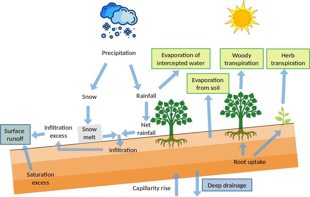
Figure 3.1: Schematic representation of soil and snow pack water balance components. Subsurface lateral source/sinks and surface runon are omitted for simplicity. Green and blue boxes represent outflows corresponding to green and blue water respectively.
Taking all input and output terms, daily variations in soil water content (\(\Delta{V_{soil}}\) in mm) are then summarized as: \[\begin{equation} \Delta{V_{soil}} = (If + Lw + Cr) - (Dd + Se + Es + Tr) \tag{3.3} \end{equation}\] The water leaving the soil via surface runoff (\(Ru\)) is defined as the sum of infiltration excess (\(Ie\)) and saturation excess (\(Se\)): \[\begin{equation} Ru = Ie + Se \tag{3.4} \end{equation}\]
If we consider soil and snow pack altogether, the water balance of the whole forest becomes: \[\begin{equation} \Delta{V_{soil}} + \Delta{S_{snow}} = (P + Ro + Lw + Cr) - (Dd + Ru + In + Es + Tr) \tag{3.5} \end{equation}\] Among inputs, precipitation (\(P\)) will the most relevant inflow on most instances. The liquid water fluxes contributing to blue water outflow (i.e. entering river networks or leading to ground water) are runoff (\(Ru\)) and deep drainage (\(Dd\)). Water vapor fluxes (\(Es\), \(Tr_{cohorts}\), \(Tr_{herb}\), \(Tr_{mist}\), \(In\)) contribute to total evapotranspiration, or green water (i.e. water vapor returning to the atmosphere). These are represented in Fig. 3.1 using blue/green boxes.
While the above describes the default water balance equations, variations can occur depending on specific control flags:
- If snow dynamics are considered [
snowpack], evaporation from bare soil cannot occur if there is a snow pack over the soil (i.e., if \(S_{snow}>0\) then \(Es = 0\)). - If plant water pools are considered [
rhizosphereOverlap], the soil water balance equation applies not only to the soil of the overall stand but also to the soil beneath each plant cohort. The fraction of stand area corresponding to the water pool of each cohort is used to keep the water balance at the two scales aligned. Moreover, the water balances of soils beneath the different plant cohort are more or less correlated depending on the degree of rhizosphere overlap. - If soil flows are simulated using a dual-permeability domain [
soilDomains] there are water balance equations for the soil matrix and the macropore domain. Moreover, it affects the infiltration amounts (and hence runoff), in the latter including infiltration via macropores.
3.4 Process scheduling
For every day to be simulated, the model performs the following steps:
- Update leaf area values according to the phenology of species and recalculate radiation extinction (sections 4.1 and 4.2).
- Determine rainfall interception loss (\(In\)) and net rainfall (\(Pr_{net}\)) (section 5.3). The amount of water reaching the soil surface from the rainfall event is the sum of net rainfall (\(Pr_{net}\)) and surface runon (\(Ro\)), if given. If snow dynamics are included, increase snow pack from snow precipitation (\(Ps\)) and decrease it following snow melt (\(Sm\)) (section 5.2).
- Determine bare soil evaporation (\(Es\)), if snow is not present (section 5.4), and herbaceous layer transpiration (\(Tr_{herb}\); section 5.5) if required.
- Determine plant cohort transpiration (\(Tr_{cohorts}\)), including hydraulic redistribution, and photosynthesis (chapter 6). Update plant water potential (\(\Psi_{plant}\)) and plant drought stress for each plant cohort. If necessary, determine mistletoe transpiration (\(Tr_{mistletoe}\)) and the corresponding additional soil water uptake (section 6.1.6).
- Determine rainfall infiltration (section 5.6) and vertical water movement within the soil (section 5.7), while considering soil layer source/sinks from snow melt, bare soil evaporation and herbaceous layer transpiration and water uptake/redistribution by plant cohorts. This updates soil moisture and returns infiltration (\(If\)), runoff (\(Ru\)) and deep drainage (\(Dd\)).
- If fire hazard calculations are requested, estimate live and dead fuel moisture and potential fire behaviour (chapter 26).
The set of steps corresponds to simulations if plant water pools are not considered, so that only the water balance of the overall soil matters. If plant water pools are considered, steps 1, 2 and 6 are the same, because they apply to the whole forest stand. However, steps 3 is performed for each water pool separately because it depends on antecedent soil moisture. Step 4 also involves defining plant water uptake from different plant water pools depending on the proportion of fine roots of each plant cohort in each pool (see 6.1.5). Step 5 is also performed on the soil corresponding to each pool, and the resulting infiltration, runoff and drainage estimates are averaged at the stand level. Finally, the soil moisture of the overall soil is estimated by averaging the soil moisture of water pools.
3.5 Inputs and outputs
3.5.1 Soil, vegetation and meteorology
Soil
Soil input requirements are fully described in section 2.3.
Vegetation
Vegetation input requirements are fully described in section 2.4. Tree, shrub and herb cohorts do not need to be characterized with different variables in soil water balance calculations, since all living plant cohorts have a \(LAI\) value. In most cases, users only need to estimate the leaf area index corresponding to live leaves, i.e. \(LAI_{live}\), because normally at the starting point all leaves are expanded (i.e. \(LAI_{\phi} = LAI_{live}\)) and one can assume no dead leaves in the canopy (i.e., \(LAI_{dead} = 0\)). Vegetation characteristics stay constant during simulations using function spwb(), although the actual expanded leaf area (\(LAI_{\phi}\)) and dead leaf area (\(LAI_{dead}\)) may vary is the species is winter deciduous. For each plant cohort with hemi-parasitic (mistletoe) plants living on crowns, a corresponding value of mistletoe leaf area index (\(LAI_{mistletoe}\)) needs to be defined.
Meteorology
The minimum weather variables required to run the model are min/max temperatures (\(T_{min}\) and \(T_{max}\)), min/max relative humidity (\(RH_{min}\) and \(RH_{max}\)), precipitation (\(P\)) and solar radiation (\(Rad\)). Wind speed (\(u\)) is also needed, but the user may use missing values if not available (a default value will be used in this case). Wind speed is assumed to have been measured at a specific height above the canopy (by default at 2 m). Atmospheric \(CO_2\) concentration (\(C_{atm}\)) may also be specified, but if missing a default constant value is assumed, which is taken from the control parameters. Definitions and units of these variables were given in section 2.5.
3.5.2 Vegetation functional parameters
The following sets of functional parameters should be supplied for each plant cohort. In practice, they are normally estimated from the species-specific parameter table and imputation of missing values (see A). Functional attributes are filled for each cohort \(i\) by function spwbInput() from species identity (i.e. \(SP_i\)). However, different parameters can be specified for different cohorts of the same species if desired (see section 2.4.4).
A first set of functional parameters refers to leaf phenology (paramsPhenology):
| Symbol | Units | R | Description |
|---|---|---|---|
PhenologyType |
Leaf phenology type (oneflush-evergreen, progressive-evergreen, winter-deciduous, winter-semideciduous) | ||
| \(LD\) | years | LeafDuration |
Average duration of leaves (in years). |
| \(t_{0,eco}\) | days | t0gdd |
Date to start the accumulation of degree days. |
| \(S^*_{eco}\) | \(^{\circ} \mathrm{C}\) | Sgdd |
Degree days corresponding to leaf budburst (see section 4.1.2). |
| \(T_{eco}\) | \(^{\circ} \mathrm{C}\) | Tbgdd |
Base temperature for the calculation of degree days to leaf budburst (see section 4.1.2). |
| \(S^*_{sen}\) | \(^{\circ} \mathrm{C}\) | Ssen |
Degree days corresponding to leaf senescence (see section 4.1.3). |
| \(Ph_{sen}\) | hours | Phsen |
Photoperiod corresponding to start counting senescence degree-days (see section 4.1.3). |
| \(T_{sen}\) | \(^{\circ} \mathrm{C}\) | Tbsen |
Base temperature for the calculation of degree days to leaf senescence (see section 4.1.3). |
| \(x_{sen}\) | {0,1,2} | xsen |
Discrete values, to allow for any absent/proportional/more than proportional effects of temperature on senescence (see section 4.1.3). |
| \(y_{sen}\) | {0,1,2} | ysen |
Discrete values, to allow for any absent/proportional/more than proportional effects of photoperiod on senescence (see section 4.1.3). |
A second set of parameters relate to light extinction and water interception (paramsInterception):
| Symbol | Units | R | Description |
|---|---|---|---|
| \(k_{PAR}\) | kPAR |
PAR extinction coefficient (see section 4.2). | |
| \(s_{water}\) | \(mm\,H_2O·LAI^{-1}\) | g |
Crown water storage capacity (i.e. depth of water that can be retained by leaves and branches) per LAI unit (see section 5.3). |
A third set includes parameters related to plant anatomic and morphological attributes (paramsAnatomy):
| Symbol | Units | R param | Description |
|---|---|---|---|
| \(1/H_{v}\) | \(m^2 \cdot m^{-2}\) | Al2As |
Ratio of leaf area to sapwood area |
| \(RLR\) | \(m^2 \cdot m^{-2}\) | Ar2Al |
Fine root area to leaf area ratio |
| \(SLA\) | \(m^2 \cdot kg^{-1}\) | SLA |
Specific leaf area |
| \(\rho_{leaf}\) | \(g \cdot cm^{-3}\) | LeafDensity |
Leaf tissue density |
| \(\rho_{wood}\) | \(g \cdot cm^{-3}\) | WoodDensity |
Wood tissue density |
| \(\rho_{fineroot}\) | \(g \cdot cm^{-3}\) | FineRootDensity |
Fine root tissue density |
| \(SRL\) | \(cm \cdot g^{-1}\) | SRL |
Specific root length |
| \(RLD\) | \(cm \cdot cm^{-3}\) | RLD |
Fine root length density (i.e. density of root length per soil volume) |
| \(r_{6.35}\) | r635 |
Ratio between the weight of leaves plus branches and the weight of leaves alone for branches of 6.35 mm |
A fourth set of parameters are related to transpiration and photosynthesis (paramsTranspiration):
| Symbol | Units | R | Description |
|---|---|---|---|
| \(g_{swmin}\) | \(mol\, H_2O \cdot s^{-1} \cdot m^{-2}\) | Gwmin |
Minimum stomatal conductance to water vapour |
| \(T_{max, LAI}\) | Tmax_LAI |
Empirical coefficient relating LAI with the ratio of maximum transpiration over potential evapotranspiration (see section 6.1.1). | |
| \(T_{max, sqLAI}\) | Tmax_LAIsq |
Empirical coefficient relating squared LAI with the ratio of maximum transpiration over potential evapotranspiration (see section 6.1.1). | |
| \(\Psi_{extract}\) | \(MPa\) | Psi_Extract |
The water potential at which plant transpiration is 50% of its maximum (see section 6.1.2). |
| \(c_{extract}\) | Exp_Extract |
Parameter of the Weibull function regulating transpiration reduction (see section 6.1.2). | |
| \(c_{leaf}\), \(d_{leaf}\) | (unitless), MPa | VCleaf_c, VCleaf_d |
Parameters of the vulnerability curve for leaf xylem |
| \(c_{stem}\), \(d_{stem}\) | (unitless), MPa | VCstem_c, VCstem_d |
Parameters of the vulnerability curve for stem xylem |
| \(WUE_{\max}\) | \(g\, C \cdot mm^{-1}\) | WUE |
Water use efficiency at VPD = 1kPa and without light or CO2 limitations (see section 6.1.7). |
| \(WUE_{PAR}\) | WUE_par |
Coefficient describing the progressive decay of WUE with lower light levels (see section 6.1.7). | |
| \(WUE_{CO2}\) | WUE_co2 |
Coefficient for WUE dependency on atmospheric CO2 concentration 6.1.7). | |
| \(WUE_{VPD}\) | WUE_vpd |
Coefficient for WUE dependency on vapor pressure deficit 6.1.7). |
A fifth (final) set of parameters are related to water storage and water relations in plant tissues (paramsWaterStorage):
| Symbol | Units | R | Description |
|---|---|---|---|
| \(LFMC_{\max}\) | % | maxFMC |
Maximum live fuel moisture content, corresponding to fine fuels (< 6.35 mm twigs and leaves). |
| \(\epsilon_{leaf}\) | MPa | LeafEPS |
Modulus of elasticity of leaves |
| \(\epsilon_{stem}\) | MPa | StemEPS |
Modulus of elasticity of symplastic xylem tissue |
| \(\pi_{0,leaf}\) | MPa | LeafPI0 |
Osmotic potential at full turgor of leaves |
| \(\pi_{0,stem}\) | MPa | StemPI0 |
Osmotic potential at full turgor of symplastic xylem tissue |
| \(f_{apo,leaf}\) | [0-1] | LeafAF |
Apoplastic fraction in leaf tissues |
| \(f_{apo,stem}\) | [0-1] | StemAF |
Apoplastic fraction in stem tissues |
| \(V_{leaf}\) | \(l \cdot m^{-2}\) | Vleaf |
Leaf water capacity per leaf area unit |
| \(V_{sapwood}\) | \(l \cdot m^{-2}\) | Vsapwood |
Sapwood water capacity per leaf area unit |
3.5.3 Control parameters
Control parameters modulate the overall behaviour of water balance simulations (see section 2.6). Most importantly, transpirationMode defines the transpiration model, which in turn defines the complexity of the water balance model. If transpirationMode = "Granier" (the default value) then the basic water balance model is used.
The other relevant control parameters for the basic water balance model are:
soilFunctions [= "SX"]: Soil water retention curve and conductivity functions, either ‘SX’ (for Saxton) or ‘VG’ (for Van Genuchten).truncateRootDistribution [= FALSE]: Boolean flag to indicate that fine root distribution is to be truncated (i.e. \(Z_{100}\) is estimated from \(Z_{95}\) when not provided).ndailysteps [= 24]: Number of steps into which each day is divided for determination of soil water balance (24 equals 1-hour intervals).max_nsubsteps_soil [= 300]: Maximum number of substeps for soil water balance solving.defaultWindSpeed [= 2.5]: Default value for wind speed (in \(m \cdot s^{-1}\)) when this is missing (only used for leaf fall, see section 4.1).defaultCO2 [=386]: Default atmospheric (abovecanopy) \(CO_2\) concentration (in micromol \(CO_2 \cdot mol^{-1}\) = ppm). This value will be used whenever \(CO_2\) concentration is not specified in the weather input.defaultRainfallIntensityPerMonth [= c(1.5, 1.5, 1.5, 1.5, 1.5, 1.5, 5.6, 5.6, 5.6, 5.6, 5.6, 1.5)]: A vector of twelve values indicating the rainfall intensity (mm/h) per month. By default synoptic storms (1.5 mm/h) are assumed between December and June, and convective storms (5.6 mm/h) are assumed between July and November (Miralles et al. 2010).snowpack [= TRUE]: Whether dynamics of snow pack are included (see section 5.2).leafPhenology [ = TRUE]: Whether leaf phenology is simulated (see section 4.1). IfFALSEthen all species are assumed to be evergreen.bareSoilEvaporation [= TRUE]: Whether evaporation from the soil surface is simulated (see section 5.4).unlimitedSoilWater [=FALSE]: Boolean flag to indicate the simulation of plant transpiration assuming that soil water is always at field capacity.unfoldingDD [= 300]: Degree-days for complete leaf unfolding after budburst has occurred (\(S_{unf}^*\); see section 4.1.2).interceptionMode [= "Gash1995"]: Infiltration model, either “Gash1995” or “Liu2001”; see section 5.3.infiltrationMode [= "GreenAmpt1911"]: Infiltration model, either “GreenAmpt1911” or “Boughton1989”; see section 5.6.soilDomains [="buckets"]: Either"buckets"(for multi-bucket model),"single"(for single-domain Richards model) and"dual"(for dual-permeability model). See 5.7.max_nsubsteps_soil [= 300]: Maximum number of substeps for soil water balance solving.fireHazardResults [= FALSE]: Boolean flag to force calculation of daily fire hazard.rhizosphereOverlap [="partial"]: A string indicating the degree of rhizosphere spatial overlap between plant cohorts:"none"- no overlap (independent water pools)."partial"- partial overlap determined by soil moisture."total"- total overlap (plants extract from common soil pools).
verticalLayerSize [= 100]: Size of vertical layers (in cm) for the calculation of light extinction (see section 2.4.3.3).windMeasurementHeight [ = 200]: Height (in cm) over the canopy corresponding to wind measurements.stemCavitationRecovery/leafCavitationRecovery [= "rate"]: A string indicating how to model recovery of xylem conductance (see section 14.4). Allowed values are:"none"- no recovery."annual"- complete recovery every first day of the year."total"- instantaneous complete recovery."rate"- following a rate of new leaf or sapwood formation.
cavitationRecoveryMaximumRate [= 0.05]: Maximum rate of conductance recovery (see section 6.2.2).lfmcComponent [= "fine"]: Plant component used to estimate LFMC, either “leaf” or “fine” (for fine fuel) (see section 10.3.4).mistletoeParams: A list with the following elements:kPAR [= 0.5]: Mistletoe light extinction coefficient.g [= 0.8]: Mistletoe water storage capacity per LAI unit.Tmax_LAI [= 0.134]: Empirical coefficient relating mistletoe LAI with the ratio of maximum transpiration over potential evapotranspiration.Tmax_LAIsq [= -0.006]: Empirical coefficient relating squared mistletoe LAI with the ratio of maximum transpiration over potential evapotranspiration.Gs_P50_Baldocchi [= -2.5]: Water potential corresponding to 50% reduction of mistletoe stomatal conductance (i.e. \(\Psi50_{gs, bald, mistletoe}\)).Gs_slope_Baldocchi [= 30]: Rate of decrease in mistletoe stomatal conductance at Gs_P50 (i.e. \(slope_{gs, bald, mistletoe}\)).
defoliationParams: A list with the following elements:cavitationInducedDefoliation [= TRUE]: Whether leaf hydraulic impairment induces defoliation.criticalLeafPLC [= 0.88]: Level of PLC (a proportion) corresponding to 50 % crown defoliation.cvLeafP50 [= 10.0]: Coefficient of variation (in percent) of leaf P50 within crown leaves.
3.5.4 Model output
Function spwb() returns a list of a class with the same name. The first four elements of this list (i.e., latitude, topography, weather and spwbInput) are simply copies of model inputs. The next element is spwbOutput, which contains the state of the input object at the end of the simulation (this can be used to perform further simulations starting with current values of state variables). The next five elements correspond to water balance flows, soil state variables, stand-level variables, plant-level and fire hazard results:
| Element | Description |
|---|---|
WaterBalance |
Climatic input and water balance flows of eq.(3.3) (i.e. net precipitation, infiltration, runoff, transpiration…). All of them in \(mm = l \cdot m^{-2}\). |
Soil |
Soil variables for each soil layer: Moisture relative to field capacity (\(W_s\)), water potential (\(\Psi_s\)) and volumetric water content (\(V_s\)). Only returned if soilResults = TRUE. |
Stand |
Stand-level variables, such as \(LAI_{\phi}\), \(LAI_{dead}\), the water retention capacity of the canopy (\(S_{canopy}\)) or the fraction of light reaching the ground (\(L^{PAR}_{ground}\) and \(L^{SWR}_{ground}\)). Only returned if standResults = TRUE. |
Plants |
Variables defined at the level of plant cohort, such as expanded leaf area (\(LAI_{\phi,i}\)), transpiration, photosynthesis, water potential, etc. Only returned if plantResults = TRUE. |
FireHazard |
Fire hazard variables (fuel moisture, rate of spread, fire potentials, etc). Only returned if fireHazardResults = TRUE. |
Elements WaterBalance, Soil, Stand and FireHazard are data frames with dates in rows and variables in columns, whereas Plants is itself a list with several data frames, with dates in rows and plant cohorts in columns:
| Element | Symbol | Units | Description |
|---|---|---|---|
LAI |
\(LAI_{\phi}\) | \(m^2 \cdot m^{-2}\) | Leaf area index (expanded). |
LAIlive |
\(LAI_{live}\) | \(m^2 \cdot m^{-2}\) | Leaf area index (live). |
AbsorbedSWRFraction |
\(f_i\) | [0-1] | Fraction of shortwave radiation absorbed. |
Transpiration |
\(Tr\) | mm | Transpiration per unit ground area. |
GrossPhotosynthesis |
\(A_{g}\) | \(g\,C \cdot m^{-2}\) | Gross photosynthesis per unit ground area. |
PlantPsi |
\(\Psi_{plant}\) | \(MPa\) | Plant water potential. |
LeafPLC |
\(PLC_{leaf}\) | [0-1] | Degree of leaf embolisation. |
StemPLC |
\(PLC_{stem}\) | [0-1] | Degree of stem embolisation. |
PlantWaterBalance |
mm | Internal daily plant water balance (balance of soil extraction and transpiration). | |
LeafRWC |
\(RWC_{leaf}\) | % | Mean leaf relative water content. |
StemRWC |
\(RWC_{stem}\) | % | Mean stem relative water content. |
LFMC |
\(LFMC\) | % | Live fuel moisture content (as percent of dry weight), corresponding to fine fuels (< 6.35 mm twigs and leaves). |
PlantStress |
\(DDS\) | [0-1] | Drought stress level suffered by each plant cohort (relative whole-plant transpiration). |
The output of simulations can be inspected using plot, shinyplot and summary functions specific to spwb objects (examples are given in the corresponding package vignette).
As it simulates water balance for only one day, function spwb_day() returns a much more reduced output. This function is most useful with advanced water balance modelling (chapter 7).
3.6 Applications
The basic water balance model is easier to parameterize and is faster the advanced water balance model. These features make it appropriate for applications that do not seek a high predictive capacity of water status at the plant level, but require robust estimates of water fluxes at the stand, landscape or regional levels. In our opinion the basic water balance model may be useful to monitor or forecast temporal variation in hydrological fluxes (i.e. evapotranspiration vs. drainage/runoff) and soil moisture in particular stands or in multiple stands across a landscape or region. Similarly, it can be used to monitor or forecast temporal variation of plant drought stress, fuel moisture and potential fire behavior in particular stands or in multiple stands across a landscape or region.
For example, Karavani et al. (2018) employed the water balance to provide sound estimates of soil moisture dynamics to predict mushroom production in a network forest stands. The model is particularly interesting to test the relationship between forest structure/composition and the water balance at the stand level or the drought stress suffered by plants, as done in Ameztegui et al. (2017) or Rolo & Moreno (2019). Finally, the model has been used to estimate green water and blue water provision at landscape to regional scales (Morán-Ordóñez et al. 2020; Roces-Díaz et al. 2021; Sánchez-Dávila et al. 2024, 2026).