Chapter 9 Radiation transfer
Radiation transfer is not the same throughout the day, but changes with solar hour. This is represented using \(\beta\), the solar elevation angle (see section 4.3 of the reference manual for package meteoland).
In the previous chapter we detailed sub-daily variation in temperature, direct radiation and diffuse short-wave radiation. Here we deal with the absorption of diffuse and direct shortwave radiation through the canopy as well as the long-wave radiation balance for canopy layers and the soil layer. These are necessary to estimate the different components of the canopy and soil energy balances (see eqs. (7.3), (7.4) and (7.5)) as well as to determine leaf energy balance, transpiration and photosynthesis (chapters 11 and 12). Short-wave radiation transfer can be determined for all sub-daily steps once the variation of atmospheric inputs are known. In contrast, the long-wave radiation (LWR) balance for any surface depends on its temperature and therefore, net LWR for canopy and soil layers need to be determined at each sub-daily step after closing the energy balance of the previous step (see chapter 13).
The vertical distribution of leaves in the stand is a key element of radiation transfer. As explained in section 2.4.3.3, the canopy is divided into vertical layers (whose size is determined by the control parameter verticalLayerSize), and the expanded and dead leaf area index of each cohort within each layer is determined. Let \(l\) be the number of canopy layers, \(c\) the number of plant cohorts, and \(LAI_{all,i,j} = LAI_{\phi,i,j}+LAI_{dead,i,j}\) be the leaf area index of cohort \(i\) in layer \(j\).
9.1 Short-wave radiation
In section 8.2 we explained how the model estimates instantaneous and direct/diffuse SWR and PAR at the top of the canopy. Given an input direct and diffuse short-wave irradiance at the top of the canopy, the amount of light absorbed by sunlit leaves, shade leaves and the soil follows the model of Anten & Bastiaans (2016), which we detail in the following subsections.
9.1.1 Direct and diffuse irradiance across the canopy
The average irradiance reaching the top of each canopy layer \(j\) is calculated separately for direct beam and diffuse radiation (the same equations are valid for SWR or PAR, but with different coefficients): \[\begin{eqnarray} I_{beam,j} &=& (1 - \gamma_i) \cdot I_{beam} \cdot \exp\left[ \sum_{h=j+1}^{l}{\sum_{i}^{c}{-k_{b,i}\cdot \alpha_i^{0.5}\cdot LAI_{all,i,h}}}\right]\\ I_{dif,j} &=& (1 - \gamma_i) \cdot I_{dif} \cdot \exp\left[ \sum_{h=j+1}^{l}{\sum_{i}^{c}{-k_{d,i}\cdot \alpha_i^{0.5}\cdot LAI_{all,i,h}}}\right] \end{eqnarray}\] where \(I_{beam}\) and \(I_{dif}\) are the direct and diffuse irradiance at the top of the canopy (in \(W \cdot m^{-2}\)), \(\gamma_i\) is the leaf reflectance (\(\gamma_{SWR, i}\) is an input parameter, whereas \(\gamma_{PAR, i} = 0.8 \cdot \gamma_{SWR, i}\)), \(k_{b,i}\) is the extinction coefficient of cohort \(i\) for direct light, \(k_{d,i}\) is the extinction coefficient of cohort \(i\) for diffuse light (i.e. \(k_{PAR,i}\) or \(k_{SWR,i}\)) and \(\alpha_i\) is the absorbance coefficient (\(\alpha_{SWR,i}\) is an input parameter, whereas \(\alpha_{PAR,i} = \alpha_{SWR,i} \cdot 1.35\)).
Plant leaves are not disposed horizontally but have an inclination (i.e. a leaf angle \(\lambda_{leaf}\)) which may change from one species to the other and determines radiation extinction along with solar elevation. The extinction coefficient for direct light, \(k_b\), depends on the leaf angle (\(\lambda_{leaf}\)) and the solar elevation angle (\(\beta\)), as described in Sellers (1985). First \(\lambda_{leaf}\) is used to determine \(\chi_{leaf}\), a parameter describing the departure of leaf angle distribution from the spherical distribution (which assumes all angles as equally probable):
\[\begin{equation} \chi_{leaf}(\lambda_{leaf}) = 2.0 \cdot \cos(\lambda_{leaf}) - 1.0 \end{equation}\] \(\chi_{leaf}\) equals 0 for +1 for horizontal leaves (i.e. for \(\lambda_{leaf} = 0\) degrees), 0 for random leaves (i.e. for \(\lambda_{leaf} = 60\) degrees) and -1 for vertical leaves (i.e. for \(\lambda_{leaf} = 90\) degrees). \(\chi_{leaf}\) and \(\beta\) are then used to estimate \(G_b\) the relative projected area of leaves in the direction of the solar beam:
\[\begin{equation} G_b(\lambda_{leaf}, \beta) = \phi_1 + \phi_2 \cdot \sin(\beta); \end{equation}\] where \(\phi_1 = 0.5 - 0.633\cdot \chi_{leaf} - 0.33\cdot \chi_{leaf}^2\) and \(\phi_2 = 0.877 \cdot (1 - 2\cdot \phi_1)\) for \(-0.4 \leq \chi_{leaf} \leq 0.6\). Finally, \(k_b\) is estimated as:
\[\begin{equation} k_b = \frac{G_b(\lambda_{leaf}, \beta)}{\sin(\beta)} \end{equation}\]
The calculations can be illustrated with function light_directionalExtinctionCoefficient():
solarElevation <- 40 # in degrees
meanLeafAngle <- 60 # in degrees
sdLeafAngle <- 20

## Parameters of the beta distribution
beta <- light_leafAngleBetaParameters(meanLeafAngle*(pi/180), sdLeafAngle*(pi/180))
beta
## p q
## 2.333333 1.166667## Direct beam extinction coefficient for solar elevation
kb <- light_directionalExtinctionCoefficient(beta["p"], beta["q"], solarElevation*(pi/180))
kb## [1] 0.76968129.1.2 Sunlit and shade leaves
It is generally accepted that sunlit and shade leaves need to be treated separately for photosynthesis calculations (De Pury & Farquhar 1997). This separation is necessary because photosynthesis of shade leaves has an essentially linear response to irradiance, while photosynthesis of leaves in sunflecks is often light saturated and independent of irradiance. The proportion of sunlit leaves, i.e. leaves in a canopy layer \(j\) that the direct light beams (sunflecks) reach is: \[\begin{equation} f_{SL, j} = \exp\left( \sum_{k>j}^{l}{\sum_{i}^{c}{-k_{b,i} \cdot LAI_{all,i,k}}}\right) \cdot \exp\left( \sum_{i}^{c}{-k_{b,j} \cdot 0.5\cdot LAI_{all,i,j}}\right) \end{equation}\] where it is assumed that only half the leaf area of layer \(j\) contributes self-shading. Note that since \(k_b\) depends on the time of the day, also \(f_{SL_j}\) may be different depending on the solar hour. From fraction \(f_{SL,j}\) we can derive the (expanded) leaf area of each layer that is affected by direct light beams (i.e. the amount of sunlit and shade leaves): \[\begin{eqnarray} LAI_{sunlit,i,j} &=& f_{SL,j} \cdot LAI_{\phi,i,j} \\ LAI_{shade,i,j} &=& (1 - f_{SL,j}) \cdot LAI_{\phi,i,j} \tag{9.1} \end{eqnarray}\]
As an example we will consider a canopy of one species of LAI = 2, divided into ten layers with constant leaf density:
LAI = 2
nlayer = 10
LAIlayerlive = matrix(rep(LAI/nlayer,nlayer),nlayer,1)
LAIlayermax = matrix(rep(LAI/nlayer,nlayer),nlayer,1)
LAIlayerdead = matrix(0,nlayer,1)
LAIlayermist = matrix(0,nlayer,1)
We will also define the coefficients of diffuse extinction, leaf absorbance and leaf reflection for PAR and SWR:
These definitions, and that of direct extinction coefficient, lead to a percentage of the above-canopy irradiance reaching each layer (Anten & Bastiaans 2016). Extinction of direct radiation also defines the proportion of leaves of each layer that are affected by sunflecks (i.e. the proportion of sunlit leaves). Both outcomes are illustrated in the figure below:
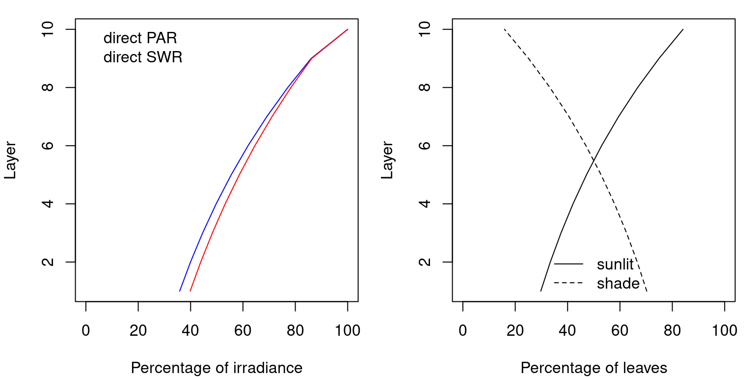
Figure 9.1: The left panel shows irradiance per layer of diffuse and direct PAR and SWR assuming a LAI of 2 equally distributed among layers (see function light_layerIrradianceFraction()). The right panel shows the corresponding proportions of sunlit and shade leaves in each layer (see function light_layerSunlitFraction()).
9.1.3 Short-wave radiation absorbed by canopy elements
The amount of absorbed diffuse radiation per leaf area unit of cohort \(i\) within a given canopy layer \(j\) is calculated as: \[\begin{equation} \Phi_{dif,i,j} = I_{dif,j} \cdot k_{d,i} \cdot \alpha_i^{0.5} \exp\left[ \sum_{h}^{c}{-k_{d,h}\cdot \alpha_i^{0.5}\cdot 0.5\cdot LAI_{all,h,j}}\right] \end{equation}\]
The amount of absorbed scattered beam radiation per leaf area unit of cohort \(i\) within a given canopy layer \(j\) is calculated as: \[\begin{eqnarray} \Phi_{sca,i,j} &=& I_{b,j} \cdot k_{b,j} \cdot (A - B) \\ A &=& \alpha_i^{0.5}\cdot \exp \left( \sum_{h}^{c}{-k_{b,i}\cdot \alpha_i \cdot 0.5\cdot LAI_{all,h,i}}\right) \\ B &=& \frac{\alpha_i}{(1-\gamma_i)}\cdot \exp\left( \sum_{h}^{c}{-k_{b,i}\cdot 0.5\cdot LAI_{all,h,i}}\right) \end{eqnarray}\]
Finally, the direct radiation absorbed by a unit of sunlit leaf area of cohort \(i\) in a canopy layer \(j\) does not depend on the position of the canopy layer and is: \[\begin{equation} \Phi_{dir,i,j} = I_{beam} \cdot \alpha_i \cdot k_{b,i} \end{equation}\]
Once these components are known, the amount of light absorbed by sunlit/shaded foliage of cohort \(i\) in layer \(j\) per leaf area unit (\(\Phi_{sunlit,i,j}\) and \(\Phi_{shade,i,j}\), respectively) is: \[\begin{eqnarray} \Phi_{sunlit,i,j} &=& \Phi_{dif,i,j} + \Phi_{sca,i,j} + \Phi_{dir,i,j} \\ \Phi_{shade,i,j} &=& \Phi_{dif,i,j} + \Phi_{sca,i,j} \tag{9.2} \end{eqnarray}\]
Let us show how all this works in an example. Regarding incoming light, we assume the following direct and diffuse irradiance at the top of the canopy:
Solar elevation is the angle between the sun and the horizon (i.e. the complement of the zenith angle). Under these conditions, and for the same canopy used for fig. 9.1, the amount of PAR and SWR absorbed per unit of leaf area at each canopy layer is (Anten & Bastiaans 2016):
ZF <- c(0.178, 0.514, 0.308) ##Standard overcast sky
Zangles <- c(15.0, 45.0, 75.0);
KDIFF <- matrix(NA, 3, 1);
for(k in 1:3){
  KDIFF[k,1] <- light_directionalExtinctionCoefficient(beta["p"], beta["q"], Zangles[k]*(pi/180.0));
}
KDIFF
## [,1]
## [1,] 1.9888914
## [2,] 0.6926432
## [3,] 0.4853480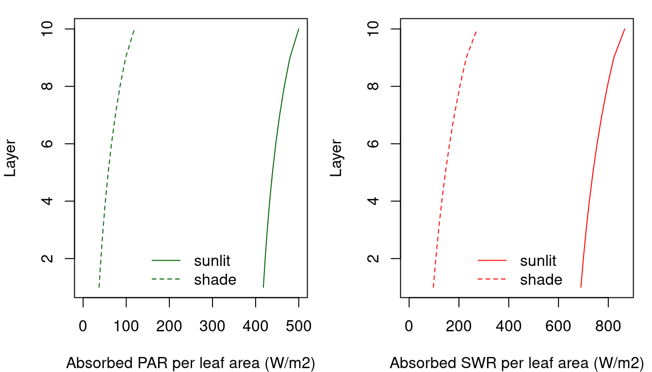
Figure 9.2: PAR (left) and SWR (right) absorbed per unit of sunlit/shade leaf area at each canopy layer (\(I_{sunlit,i,j}\) and \(I_{shade,i,j}\), respectively;see function light_cohortSunlitShadeAbsorbedRadiation()).
The SWR absorbed per ground area unit by sunlit and shade foliage of cohort \(i\) in canopy layer \(j\) is: \[\begin{eqnarray} K_{abs,sunlit,i,j} &=& \Phi_{sunlit,i,j} \cdot LAI_{sunlit,i,j} \\ K_{abs,shade,i,j} &=& \Phi_{shade,i,j} \cdot LAI_{shade,i,j} \end{eqnarray}\] The previous quantities can be aggregated across cohorts or layers. The SWR absorbed per ground area unit by cohort \(i\) (\(K_{abs,i}\)) is found using: \[\begin{equation} K_{abs,i} = \sum_j^l{K_{abs,sunlit,i,j} + K_{abs,shade,i,j}} = K_{abs,sunlit,i} + K_{abs,shade,i} \end{equation}\] where \(K_{abs,sunlit,i}\) and \(K_{abs,shade,i}\) are the SWR absorbed per ground area unit by sunlit and shade foliage, respectively, of cohort \(i\). Similarly, the SWR absorbed by canopy layer \(j\) (\(K_{abs,j}\)) is found using: \[\begin{equation} K_{abs,j} = \sum_i^c{K_{abs,sunlit,i,j} + K_{abs,shade,i,j}} \end{equation}\] and the SWR absorbed by the whole canopy (\(K_{abs,ca}\)) is: \[\begin{equation} K_{abs,ca} = \sum_j^l{K_{abs,j}} = \sum_i^c{K_{abs,i}} =\sum_i^c{\sum_j^l{K_{abs,sunlit,i,j} + K_{abs,shade,i,j}}} \end{equation}\]
9.1.4 Short-wave radiation absorbed by the soil
The instantaneous shortwave radiation reaching the soil is calculated separately for direct beam and diffuse radiation: \[\begin{eqnarray} I_{beam, soil} &=& I_{beam} \cdot \exp\left[ \sum_{h=j+1}^{l}{\sum_{i}^{c}{-k_{b,i}\cdot \alpha_i^{0.5} \cdot LAI_{all,i,h}}}\right]\\ I_{dif, soil} &=& I_{dif} \cdot \exp\left[ \sum_{h=j+1}^{l}{\sum_{i}^{c}{-k_{d,i}\cdot LAI_{all,i,h}}}\right] \end{eqnarray}\] where \(I_{beam}\) and \(I_{dif}\) are the direct and diffuse irrradiance at the top of the canopy, \(k_{b,i}\) is the extinction coefficient of cohort \(i\) for direct light and \(k_{d,i}\) is the extinction coefficient of cohort \(i\) for diffuse SWR. From these, the SWR absorbed by the soil (\(K_{abs,soil}\)) is found by: \[\begin{equation} K_{abs,soil} = (1 - \gamma_{SWR, soil})\cdot (I_{beam, soil} + I_{dif, soil}) \end{equation}\] where \(\gamma_{SWR, soil} = 0.10\) is the SWR reflectance (10% albedo) of the soil.
9.2 Long-wave radiation
Long-wave radiation (LWR) transfer within the canopy is based on the SHAW model (Flerchinger et al. 2009).
9.2.1 Long-wave radiation balance by canopy layers
Assume canopy layers are ordered from \(j=1\) (in contact with the soil) to \(j=l\) (in contact with the atmosphere above the boundary layer). The procedure first calculates downward LWR below each canopy layer, \(L_{down,j}\), from \(j=l\) to \(j=1\). The downward LWR below layer \(j\) is calculated as: \[\begin{equation} L_{down,j} = \tau_{j} \cdot L_{down,j+1} + (1 - \tau_j) \cdot \epsilon_{can} \cdot \sigma \cdot (T_{air,j}+273.16)^{4} \end{equation}\] where \(L_{down,j+1}\) is the downward LWR of the layer above (\(L_{atm}\) in the case of \(j=l\)), \(T_{air,j}\) is the air temperature of layer \(j\), \(\tau_j\) is the diffuse transmissivity of layer \(j\), \(\sigma = 5.67 \cdot 10^{-8}\,W \cdot K^{-4}\cdot m^{-2}\) is the Stephan-Boltzmann constant and \(\epsilon_{can} = 0.97\) is the canopy emmissivity. Diffuse transmissivity values are defined by cohort \(i\) and layer \(j\) using: \[\begin{equation} \tau_{i,j} = \exp{(-k_{LWR} \cdot LAI_{all,i,j})} \end{equation}\] where \(k_{LWR} = 0.7815\) is the extinction coefficient for LWR. The transmissivity of layer \(j\) is simply \(\tau_{j} = \sum_i^c {\tau_{i,j}}\). Once we know \(L_{down,1}\) we can calculate the upwards LWR from the soil (\(L_{up,s}\)) using: \[\begin{equation} L_{up,soil} = (1- \epsilon_{soil}) \cdot L_{down,1} + \epsilon_{soil} \cdot \sigma \cdot (T_{soil,1}+273.16)^{4} \end{equation}\] where \(T_{soil, 1}\) is the temperature of the topmost soil layer and \(\epsilon_{soil} = 0.97\) is the soil emmissivity. Now we calculate upward LWR from \(j=1\) to \(j=J\): \[\begin{equation} L_{up,j} = \tau_{j} \cdot L_{up,j-1} + (1 - \tau_j) \cdot \epsilon_{can} \cdot \sigma \cdot (T_{air,j}+273.16)^{4} \end{equation}\] where \(L_{up,j-1}\) is the downward LWR of the layer below (\(L_{up,soil}\) in the case of \(j=1\)). Once we have downward and upward LWR fluxes, we can estimate the net LWR absorbed within canopy layer \(j\) using: \[\begin{equation} L_{net,j} = \epsilon_{can} \cdot (1 - \tau_j) \cdot (L_{down,j} + L_{up,j} - \sigma \cdot (T_{air,j}+273.16)^{4}) \end{equation}\]
9.2.2 Net long-wave radiation of the whole canopy and the soil
Net LWR can be aggregated at the scale of the whole canopy. The net LWR of the whole canopy (\(L_{net,can}\)) is simply the sum across layers of net LWR: \[\begin{equation} L_{net,can} = \sum_j^l{L_{net,j}} \end{equation}\] whereas the net LWR of the soil (\(L_{net,soil}\)) is: \[\begin{equation} L_{net,soil} = \epsilon_{soil} \cdot (L_{down,1} - \sigma \cdot (T_{soil,1}+273.16)^{4}) \end{equation}\]
9.2.3 Long-wave radiation balance by plant cohorts
The net LWR per leaf area unit absorbed within canopy layer \(j\) can also be decomposed among plant cohorts. The net LWR of cohort \(i\) in layer \(j\) is found using the relative proportion of light absorbed by the cohort (i.e. the complement of its diffuse transmissivity): \[\begin{equation} L_{net,i, j} = L_{net,j} \cdot \frac{1-\tau_{i,j}}{\sum_h{1-\tau_{h,j}}} \end{equation}\] from which we can estimate \(L_{net,sunlit,i}\) and \(L_{net,shade,i}\), the average net LWR per leaf area unit for sunlit and shade leaves of cohort \(i\), respectively: \[\begin{equation} L_{net,sunlit,i} = \frac{\sum_j^l{L_{net,i, j} \cdot LAI_{sunlit,i,j}}}{\sum_j^l{LAI_{sunlit,i,j}}} \,\,\,\, L_{net,shade,i} = \frac{\sum_j^l{L_{net,i, j} \cdot LAI_{shade,i,j}}}{\sum_j^l{LAI_{shade,i,j}}} \end{equation}\]