Chapter 22 Seed dispersal
This chapter describes the seed dispersal sub-model implemented in functions fordyn_scenario() and fordyn_land() of package medfateland (Fig. 1.3).
22.1 Design principles
Given their sessile lifestyle, dispersal is the only process through which plants can spread in a landscape. Different parts of plants can be dispersed (seeds, fruits, branches or even the entire plant), but here it is assumed that seeds are the dispersed elements. Mathematically, dispersal can be addressed via process-based models (e.g. Nathan et al. (2001)). However, it is more commonly addressed via empirical dispersal kernels, which describe the statistical distribution of dispersal distances in a population (Nathan et al. 2012). More specifically, the dispersal kernel is a probability density function describing the distribution of post-dispersal locations relative to a source point. While many different equations can be used and compared to describe dispersal (Nathan et al. 2012), here we focus on the exponential power kernel proposed by Clark et al. (1998), which has shown a good performance compared to other kernels (Bullock et al. 2017) and has been used for other dynamic vegetation models (Snell 2014). The kernel is isotropic, meaning that is equal in all directions. Therefore, one can consider dispersal either from source or sink locations.
When implementing a dispersal kernel in a dynamic forest simulation model, an important issue to overcome is the fact that forest stands in the target landscape are often separated by distances that are larger (e.g. 500 m, 1 km or even more) than the average area that they represent (normally forest plots have a radius between 10 and 25 m). This entails that there is a uncertainty in the model regarding the presence of seed sources from forest stands at distances between the two scales. In other words, the model does not know whether there are forest patches that can act as seed sources, between a given target forest stand and its nearest neighbors (Fig. 22.1). Ignoring this fact can lead to underestimating colonization. We address this issue by considering that seed sources from unavailable forest stands can be estimated from the set of stands that are represented in the data set, using weights inverse to their distance to the location of the unavailable stand. This is illustrated in Fig. 22.1 below with the area with unavailable stands in grey and distances represented using red and black arrows:
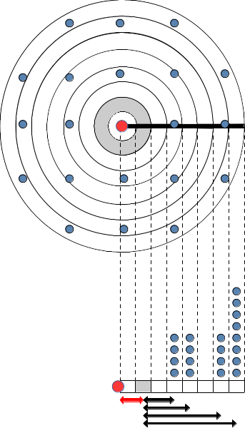
Figure 22.1: Example of sparse forest stand distribution and how to deal with dispersal in this situation. The target stand where seed rain is to be determined is represented using a red dot. Blue dots are the remaining forest stands. The upper figure shows the spatial distribution of stands, whereas the figure below represents the number of stands per distance classes. In both cases, grey is used to identify an area with unavailable data.
22.2 Process scheduling
Seed dispersal is considered once a year. Process scheduling in the dispersal sub-model is rather straightforward:
22.3 Process details
The exponential power kernel depends on species-specific parameters \(Disp_{dist}\) and \(Disp_{shape}\) and is calculated for a given distance \(r\) using (Clark et al. 1998): \[\begin{equation} f(r) = \frac{1}{N} \cdot \exp \left[ - \left( \frac{r}{Disp_{dist}} \right)^{Disp_{shape}} \right] \end{equation}\] where \(N\) is the normalizing constant: \[\begin{equation} N = \frac{2\cdot \pi \cdot Disp_{dist}^2 \cdot \Gamma(2/Disp_{shape})}{Disp_{shape}} \end{equation}\] and \(\Gamma()\) is the Gamma function.
Let \(i\) be the stand corresponding to seed sink location (e.g. the red dot in Fig. 22.1). We begin by computing the geographic distances between \(i\) and all the other stands using geographic coordinates \(x\) and \(y\) (assuming these are in meters). \[\begin{equation} d(i,j) = \sqrt{(x_i - x_j)^2 + (y_i - y_j)^2} \end{equation}\]
Let us now consider a given distance value \(r > 0\) from \(i\) (e.g. the grey band in Fig. 22.1). We define the probability of choosing a given stand \(j\) for a location at this distance from \(i\) as follows: \[\begin{equation} p_i(r, j) = \frac{1}{M}\cdot \frac{1}{|r - d(i,j)|} \end{equation}\] where \(M\) is an appropriate normalizing factor so that: \[\begin{equation} \sum_{j=1}^n{p_i(r, j)} = 1 \end{equation}\] Note that this last equation assumes that the density of spatial points is even across space. If not, the sum should be lower than one.
Given the above definitions and assuming that seed bank of a given species should be refilled to 100% if and only if all plots are seed sources for that species, the percentage of seeds of species \(s\) reaching the target location \(i\), i.e. \(P_{s, i}\), is estimated using: \[\begin{equation} P_{s, i} = 100 \cdot 2 \pi \cdot \int_{r > 0}^{r_{\max}}{r \cdot f(r) \cdot \left( \sum_{j=1}^{n}{I(s, j) \cdot p_i(r,j)} \right) \cdot \delta r} \end{equation}\]
where \(r_{\max}\) is the maximum allowed dispersal distance and \(I(s,j) \in {0,1}\) is an indicator variable of the availability of seed sources of species \(s\) in stand \(j\).