Chapter 2 Model inputs

This chapter describes the inputs required by simulation models of medfate and medfateland packages. First, we describe the R structures required for the two packages. Then, we provide the details for four different kinds of inputs:

1. Vegetation existing in the forest stand. This information should be available at a level of detail appropriate for the model design, which in our case includes not only species composition and/or structure, but also functional parameters of woody plants. Vegetation structure is considered static in spwb() calls, but becomes dynamic in calls to growth() or fordyn(). Hence, in these functions the input vegetation describes the starting point.
2. Information on the physical structure of soil. Soil information is also required but, unlike vegetation, the soil physical structure is considered static.
3. Climatic forcing. Daily weather series are always required, defining the temporal extent of the simulation and the temporal variation of environmental conditions in which physical and biological processes occur.
4. Topographic information and geographic location. Topography and latitude are also required, because internal calculations of some physical variables require them.

The last section (2.6) describes additional input parameters that are used to specify global options of simulation functions.

Since preparing inputs for simulations can be daunting for most users, package medfateland provides a set of utility functions aimed at facilitating the preparation of vegetation and soil inputs, whereas package meteoland provides functions to assess daily weather over landscapes.

2.1 Input structures

2.1.1 Input structures in medfate

Package medfate deals with simulations at stand level and, hence, the data structures defined in the package are meant to encapsulate information about a target forest stands and the properties of the soil where it grows:

• S3 class soil is a data frame that is initialized using a data frame of soil physical properties, but the table includes also soil parameters and state variables. Soil objects are described in subsection 2.3.3.
• S3 class forest is a list of forest inventory data (i.e. mainly tree and shrub measurements, but can include herbaceous vegetation) corresponding to a single forest stand. Forest plot objects are described in subsection 2.4.4.
• S3 classes spwbInput and growthInput are lists containing all the vegetation parameters and state variables necessary to run water-balance simulations (function spwb() and alike) and forest growth simulations (function growth() and alike). Objects of classes spwbInput and growthInput are created using functions whose input includes a forest object and a soil object.

The figure below (Fig. 2.1) can be used to illustrate the workflow of soil/forest input creation for the main simulation functions in medfate. Note the different inputs in the case of fordyn().

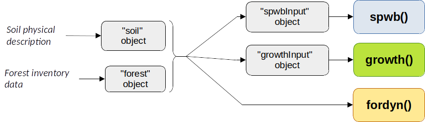
Figure 2.1: Schematic workflow of input creation for simulation functions in medfate

2.1.2 Input structures in medfateland

Spatial information for medfateland needs to be provided in sf objects (i.e. data frames with geometry, see package sf). For each forest stand to be simulated, these object must include a geometry, topographic features as well as a forest object and soil object, as illustrated in the figure below:

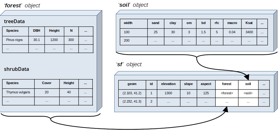
Figure 2.2: Relationship between data structures in medfate and medfateland

Non-forest (i.e. croplands or urban areas) patches may be also described, and then forest or soil objects may not be required. The actual columns required in a sf depend on the simulation function to be used, as described in the following table:

Column	Description	Use
geom	Spatial geometries (points, polygons, …)	Always required
id	Stand identifiers	Required for *_spatial(), *_spatial_day() and fordyn_scenario()
elevation	Elevation values above sea level (in m)	Always required
slope	Slope values (in degrees)	Always required
aspect	Aspect values (in degrees)	Always required
land_cover_type	Land cover type: wildland, agriculture, rock, artificial or water	Required for *_land(), optional for *_spatial() and *_spatial_day()
forest	Objects of class forest	Always required
soil	Objects of class soil	Always required
state	Objects of class spwbInput or growthInput	Optional to recover the final state of a previous simulation
meteo	Weather data frames (see 2.5)	Optional
crop_factor	Crop evapo-transpiration factor	Only required for agriculture land cover type
management_arguments	Management arguments for each stand	Optional for fordyn_spatial()
management_unit	Management unit corresponding to each stand	Required for fordyn_scenario()
represented_area_ha	Area represented by each stand, in hectares	Required for fordyn_scenario()
depth_to_bedrock	Depth to bedrock (mm).	Required for *_land()
bedrock_conductivity	Bedrock (saturated) conductivity (in m·day-1).	Required for *_land()
bedrock_porosity	Bedrock porosity ([0-1]).	Required for *_land()
snowpack	Snow water equivalent content of the snowpack (mm).	Required for *_land()
aquifer	Water content of the aquifer in each cell.	Required for *_land()

2.2 Latitude and topography

Topography has a relatively small direct influence in medfate simulations, because most topographic effects are assumed to be taken into account in the estimation of weather inputs. Nonetheless, elevation in meters is needed to estimate atmospheric pressure and air density (see 2.5), whereas aspect (in degrees from North) and slope (also in degrees) are needed in addition to latitude (also in degrees North) to estimate sunrise/sunset hours and potential radiation. Topographic variables should be readily accessible for users having access to a digital elevation model of the target area.

2.3 Soil description

Soils are described in medfate using \(S > 1\) different soil layers (\(s \in \{1, 2, ..., S\}\)). Here the word soil refers to depths that plant rooting systems can reach (i.e., the critical zone), including cracks within the bedrock. The number and size of soil layers may correspond to changes in soil properties along depth, but also can be chosen to reflect differences in plant rooting depths. The physical properties of the soil are needed to estimate soil hydraulic properties and are considered static soil parameters in simulations. In contrast, soil moisture content, other variables that depend on moisture (e.g. soil water potential and soil conductivity) and soil temperature, if the soil energy balance is considered, are all soil state variables.

2.3.1 Soil physical properties

Soil physical properties, such as texture (i.e. volume percent of sand, silt and clay), organic matter content, bulk density or rock fragment content, can differ between soil layers, and this has important consequences for soil water retention capacity and soil hydraulics. Specifying layers with an elevated rock fragment content (e.g. layers of weathered rock where soil particles are scarce) may be important in seasonally-arid climates like the Mediterranean, because plants often extend their roots into cracks existing in the parent rock to access water during summer (Ruffault et al. 2013).

For each soil layer \(s\), the following physical parameters are needed:

Symbol	Units	R	Description
\(d_{s}\)	mm	widths	Width of soil layer \(s\)
\(P_{clay,s}\)	%	clay	Percent volume of clay (within soil particles fraction) in layer \(s\)
\(P_{sand,s}\)	%	sand	Percent volume of sand (within soil particles fraction) in layer \(s\)
\(OM_s\)	%	om	Percentage of organic mater per dry weight (can be missing) in layer \(s\)
\(BD_{s}\)	\(g \cdot cm^{-3}\)	bd	Bulk density in layer \(s\)
\(P_{rocks,s}\)	%	rfc	Rock fragment content as percent volume (within whole soil) in layer \(s\)

The percent volume of silt is 100% minus the percent volume of clay and sand. Whenever possible, soil physical properties should be measured in soil profiles conducted at the target forest plot (although soil profiles rarely reach rooting depths of deeply-rooted plants). Soil input data should be arranged in a data.frame with soil layers in rows and physical variables in columns (see function defaultSoilParams()). The following is an example with four soil layers:

soildf <- defaultSoilParams()
soildf

##   widths clay sand om nitrogen  bd rfc
## 1    300   25   25 NA       NA 1.5  25
## 2    700   25   25 NA       NA 1.5  45
## 3   1000   25   25 NA       NA 1.5  75
## 4   2000   25   25 NA       NA 1.5  95

Package medfateland includes a function add_soilgrids() to fetch soil information from SoilGrids.org, a global soil database currently providing soil data at 250m scale. This can be helpful to users lacking local soil measurements, but the uncertainty of SoilGrids estimates can be high for some areas and soil properties, especially soil depth and rock fragment content.

The depth of a given soil layer \(s\) (\(Z_s\); in mm) is defined as the sum of layer widths from the surface to the target layer: \[\begin{equation} Z_s = \sum_{i=1}^s{d_s} \end{equation}\] And the overall soil depth (\(Z_{soil}\); in mm) is the sum of widths across all soil layers. As the soil may include deep rocky layers, the value of \(Z_{soil}\) may be larger than the soil depth reported in soil profiles.

2.3.2 Water retention curves

The water retention curve of a soil is the relationship between volumetric soil moisture content (\(\theta\), in \(m^3 \cdot m^{-3}\) of soil, excluding rock fragments) and the corresponding soil water potential (\(\Psi\), in MPa), i.e. the amount of work that must be done per unit quantity of pure water in order to transport reversibly and isothermally an infinitesimal quantity of water from a reference pool. The shape of the water retention curve (also called the soil moisture characteristic curve) depends on physical properties (mainly texture and bulk density, but also organic matter content). Since soil layers usually differ in their physical properties they also normally have different water retention curves.

Two water retention curve models are available in medfate (fig. 2.3):

1. Saxton model: In this model, volumetric soil moisture \(\theta(\Psi)\) corresponding to a given water potential \(\Psi\) (in MPa) below field capacity (i.e., \(\Psi < \Psi_{fc}\)) is calculated using: \[\begin{equation}\theta(\Psi) = (\Psi/A)^{(1/B)}\end{equation}\] where \(A\) and \(B\) depend on the texture and, if available, organic matter in the soil. If organic matter is available, \(A\) and \(B\) are calculated from \(P_{clay}\), \(P_{sand}\) and \(OM\) following Saxton & Rawls (2006). Otherwise, they are calculated from \(P_{clay}\) and \(P_{sand}\) as indicated in Saxton et al. (1986). Volumetric changes between field capacity and saturation (i.e., \(\Psi_{fc} \leq \Psi < 0\)) are estimated using a linear function.
2. Van Genuchten model: The well known van Genuchten (1980) model is: \[\begin{equation}\theta(\Psi) = \theta_{res}+\frac{\theta_{sat}-\theta_{res}}{\left[1+ (\alpha \cdot \Psi)^n \right]^{1-1/n}}\end{equation}\] where \(\theta(\psi)\) is the water retention, \(\theta_{sat}\) is the saturated water content, \(\theta_{res}\) is the residual water content, \(\alpha\) is related to the inverse of the air entry pressure, and \(n\) is a measure of the pore-size distribution.

## Warning: A numeric `legend.position` argument in `theme()` was deprecated in ggplot2 3.5.0.
## ℹ Please use the `legend.position.inside` argument of `theme()` instead.
## This warning is displayed once every 8 hours.
## Call `lifecycle::last_lifecycle_warnings()` to see where this warning was generated.

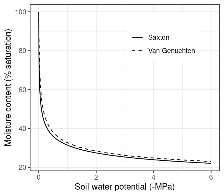
Figure 2.3: Water retention curves under the Saxton and Van Genuchten models, for the same physical attributes (25% sand, 25% clay, 50% silt and bulk density of \(1.5 g \cdot cm^{-3}\)). Parameters of the Van Genuchten curve have been estimated using pedotransfer functions given in Tóth et al. (2015).

Hydraulic conductivity governs the rate of water flow for a unit gradient in potential. It decreases sharply as soil becomes dry, and the relationship also depends on soil texture. The Saxton and Van Genuchten models also describe and parameterize the relationship between conductivity and soil water potential.

2.3.3 Soil initialization

Soil initialization is needed to estimate hydrological parameters for each soil layer \(s\) from its physical attributes. Soil initialization is done using function soil(), which returns an object of a S3 class with the same name (see 2.1.1). Simulation functions in medfate need an object of class soil to be run.

Function soil() adds the following information to the physical soil description:

Symbol	Units	R	Description
\(P_{macro}\)	%	macro	Percentage of macroporosity corresponding to each soil layers
\(\gamma_{soil}\)	\(mm \cdot day^{-1}\)	Gsoil	The maximum daily evaporation rate from soil (see 5.4)
\(\theta_{sat}\)	\(m^3 \cdot m^{-3}\)	VG_theta_sat	Volumetric soil moisture at saturation for each soil layer
\(\theta_{res}\)	\(m^3 \cdot m^{-3}\)	VG_theta_res	Residual volumetric soil moisture for each soil layer
\(n\)		VG_n	Parameter \(n\) of the Van Genuchten (1980) model for each soil layer
\(\alpha\)	\(MPa^{-1}\)	VG_alpha	Parameter \(\alpha\) of the Van Genuchten (1980) model for each soil layer
\(K_{sat}\)	\(mmol \cdot s^{-1} \cdot m^{-2} \cdot MPa^{-1}\)	Ksat	Saturated soil conductivity for each soil layer

Macroporosity values are calculated using the equations given in Stolf et al. (2011), while \(\gamma_{soil}\) is derived from texture. Parameters of the van Genuchten model for each layer are estimated from the physical description of the layer using one of two pedotransfer functions (see help for soil()):

1. Using the USDA texture classification and the average texture class parameters given by Carsel & Parrish (1988).
2. Directly from the soil texture, organic matter and bulk density, using the pedotransfer functions in Tóth et al. (2015).

Parameter \(\alpha\) of the Van Genuchten model is given in \(MPa^{-1}\), but it can be transformed to \(cm^{-1}\) using the relationship:

\[\begin{equation} 1\, cm = 0.00009804139432\,\,MPa, \end{equation}\]

which can also be applied to water potential units. Soil layer saturated conductivity (\(K_{sat}\)) is estimated using Saxton & Rawls (2006) or Saxton et al. (1986), depending on whether an estimate of organic mater is available. \(K_{sat}\) is given in physiological units \(mmol \cdot s^{-1} \cdot m^{-2} \cdot MPa^{-1}\), but they can be transformed into \(cm\cdot day^{-1}\) using:

\[\begin{equation} 1\, cm\cdot day^{-1} = 655.2934\,\,mmol \cdot s^{-1} \cdot m^{-2} \cdot MPa^{-1} \end{equation}\]

Besides defining soil parameters, function soil() also initializes soil state variables: soil moisture content, soil temperature (although set to a missing value) and water table depth. Users can edit the soil object manually (it is actually a list), for example to provide specific parameters of the Van Genuchten retention curve calibrated from soil measurements.

Saturated conductivity (\(K_{sat}\)) is corrected for bulk density (\(BD\)) of the soil layer, because compact soils have lower conductivity (Rahimi et al. 2011):

\[\begin{equation} K_{sat} = K_{sat,ref} \cdot \left( \frac{\rho_{s} - BD}{\rho_{s} - BD_{ref}} \right)^3 \end{equation}\] where \(K_{sat,ref}\) is the reference conductivity according to soil texture, \(\rho_{s} = 2.73 \,g\cdot cm^{-3}\) is density of soil particles, \(BD_{ref} = 1.2\,g\cdot cm^{-3}\) is the reference bulk density.

2.3.4 Water content and depth to saturation

The volume of water (\(V_s\) in \(mm = l \cdot m^{-2}\) of ground area) in a soil layer \(s\) is calculated from its water potential (\(\Psi_s\)) and water retention curve using: \[\begin{equation} V_s(\Psi_s) = d_s\cdot ((100-P_{rocks,s})/100)\cdot\theta_{s}(\Psi_s) \end{equation}\] where \(d_s\) is the depth of the soil layer (in mm) and \(P_{rocks,s}\) is the percentage of rock fragments. The overall volume of water in the soil (accessible by roots) is simply the sum of water content over soil layers: \[\begin{equation} V_{soil} = \sum_{s=1}^S{V_s(\Psi_s)} \end{equation}\]

A number of fixed water volumes (and their corresponding moisture) are important to remember:

• Water holding capacity (\(V_{fc, s}\), in mm) of the soil layer \(s\) is defined as the volume of water at field capacity, i.e. at \(\Psi_{fc} = -0.033\) MPa, the amount of water held in the soil after gravitational water has drained away: \[\begin{equation} V_{fc,s} = V_{s}(-0.033) = d_s\cdot ((100-P_{rocks,s})/100)\cdot\theta_{fc,s} \end{equation}\] where \(\theta_{fc,s} = \theta_s(-0.033)\) is the corresponding moisture at field capacity.
• Water content at saturation (\(V_{sat, s}\), in mm) is calculated anagolously, but replacing \(\theta_{fc,s}\) by \(\theta_{sat, s} = \theta_s(0)\), the moisture at saturation, the amount of soil moisture when all easily drained spaces between soil particles (i.e. macropores) are also filled with water.
• Water content at wilting point (\(V_{wp, s}\), in mm) is calculated replacing \(\theta_{fc,s}\) by \(\theta_{wp,s} = \theta_s(-1.5)\), the moisture at wilting point, i.e. at \(\Psi_{fc} = -1.5\) MPa, a conventional amount of soil moisture beyond which plants are assumed have problems extracting water and start to wilt. However, plants can often extract water from much drier soils.
• The amount of extractable water (in mm) is the difference between water content at field capacity and the water content at a conventional minimum water potential, which can be set at wilting point or lower values (by default at -5 MPa in medfate).

The saturated water depth (\(Z_{sat}\), in mm) is not defined (i.e. missing) when all soil layers are below field capacity. When some layers are between field capacity and saturation, depth of the saturated water is calculated as: \[\begin{equation} Z_{sat} = \sum_{s}{d_s \cdot \min\left[1,(\theta_{sat,s} - \theta(\Psi_s))/(\theta_{sat,s}-\theta_{fc,s})\right]} \end{equation}\]

2.4 Vegetation description

The representation of vegetation within a target forest stand is done in medfate primarily by means of cohorts of woody plants (i.e. trees and shrubs). A woody plant cohort represents a set of woody plants that belong to the same species (or functional group) and are more or less of the same size. For example, trees in a stand may be grouped by species and diameter class, whereas shrubs may be grouped by species and height. In practice however, plant cohorts are entities that are treated separately when modeling the forest stand. This representation in plant cohorts was chosen so that package functions can be easily applied to forest inventory data, for example from national forest surveys. The description of woody plant cohorts includes a measure of abundance of the cohort in the stand, which in the case of trees is density as stems per hectare and for shrubs is percent cover (shrubs are often multi-stemmed). The difference in measurement units for abundance is the main motivation for distinguishing between tree cohorts and shrub cohorts, rather than their size or growth form. Additionally, the description of vegetation in the forest stand may include the cover and mean height of a herbaceous layer. The presence or abundance of herbs is not always recorded in forest inventory surveys, but may be relevant vegetation component in open habitats like shrublands.

Note that one limitation of the representation of vegetation in medfate is that it is not spatially-explicit (i.e. plants cannot have explicit coordinates within forest stands) and hence spatial (horizontal) interactions between plant cannot be taken into account explicitly (but see 2.4.9).

2.4.1 Structural attributes of woody plant cohorts

A woody plant cohort \(i\) is either a tree cohort or a shrub cohort, and is defined using a set of structural attributes shown in the following table, where columns spwb, growth and fordyn indicate whether attributes are required by simulation functions spwb()/pwb(), growth() and fordyn(), respectively:

Symbol	Units	R	Description	spwb	growth	fordyn
\(SP_i\)		Species	Species identity	Y	Y	Y
\(H_i\)	\(cm\)	Height	Average tree or shrub height	Y	Y	Y
\(CR_i\)		CR	Crown ratio (i.e. ratio between crown length and plant height)	Y	Y	N
\(N_i\)	\(ind · ha^{-1}\)	N	Density of tree individuals	N	Y	Y
\(DBH_i\)	\(cm\)	DBH	Tree diameter at breast height	N	Y	Y
\(Cover_i\)	%	Cover	Shrub percent cover	N	Y	Y
\(LAI^{live}_i\)	\(m^2 \cdot m^{-2}\)	LAI_live	(Maximum) leaf area index	Y	Y	N
\(LAI^{dead}_i\)	\(m^2 \cdot m^{-2}\)	LAI_dead	(Standing) dead leaf area index	Y	Y	N
\(LAI^{\phi}_i\)	\(m^2 \cdot m^{-2}\)	LAI_expanded	Current expanded leaf area index	Y	Y	N
\(LAI^{NC}_i\)	\(m^2 \cdot m^{-2}\)	LAI_nocomp	Leaf area index assuming no competition with other plants	N	Y	N
\(Z_{50,i}\)	mm	Z50	Depth above which 50% of the fine root mass is located	Y	Y	Y
\(Z_{95,i}\)	mm	Z95	Depth above which 95% of the fine root mass is located	Y	Y	Y

Height (\(H\)) values refer to average height of individuals included in the cohort, and the same for crown ratio (\(CR\)) and diameter at breast height (\(DBH\)). While plant size (i.e. height or diameter) is relatively easy to tally, other measurements are not usually made in the field. Package medfate includes utility functions that provide estimates \(CR\) and \(LAI\) from forest inventory data (e.g. heights, DBH and density for measured trees), using allometric relationships calibrated for Catalonia, Spain (see chapter 21).

Leaf area index

\(LAI\) variables refer to one-sided leaf area of plants per surface area of the stand. Leaves standing on branches of woody plants can be alive or dead. We will call total leaf area index of a woody plant cohort \(i\) (\(LAI^{all}_{i}\)) to the sum of its dead and live (and unfolded) leaf area: \[\begin{equation} LAI^{all}_{i} = LAI^{\phi}_{i}+LAI^{dead}_{i} \end{equation}\]

For simulations not involving growth, winter-deciduous phenology is a prognosed variable, and the current level of leaves unfolded may be lower than the maximum (live) amount of leaves. In simulations involving growth, both \(LAI^{\phi}\) and \(LAI^{live}\) can change, the former due to leaf phenology (unfolding is simulated explicitly and has carbon costs) and the latter due to leaf allocation limits during plant development.

2.4.2 Structural attributes of herbaceous vegetation

The herbaceous layer of the stand is described collectively, without distinguishing among plant cohorts. Two attributes, cover and height, are required:

Symbol	Units	R	Description
\(H_{herb}\)	\(cm\)	herbHeight	Average height of herbaceous vegetation
\(Cover_{herb}\)	%	herbCover	Percent cover of herbaceous vegetation
\(LAI_{herb}\)	\(m^2 \cdot m^{-2}\)	LAI_herb	Leaf area index of herbaceous vegetation

Leaf area index of herbaceous layer (\(LAI_{herb}\)), is normally estimated from \(H_{herb}\) and \(Cover_{herb}\), but could be directly prescribed by the user. Rooting depth parameters are not needed for herbaceous vegetation, which is assumed to extract water from the topmost soil layer. Note that neither phenology or growth/senescence processes are modelled in the case of herbaceous vegetation.

2.4.3 Leaf area index of the forest stand

If there are \(c\) woody plant cohorts, the leaf area index corresponding to living leaves, unfolded leaves and dead leaves can be aggregated across cohorts using:

\[\begin{eqnarray} LAI^{live}_{woody} &=& \sum_{i=1}^c{LAI_{i}^{live}} \\ LAI^{\phi}_{woody} &=& \sum_{i=1}^c{LAI_{i}^{\phi}} \\ LAI^{dead}_{woody} &=& \sum_{i=1}^c{LAI_{i}^{dead}} \end{eqnarray}\]

We can also estimate the overall leaf area index of woody plant cohorts (\(LAI^{all}_{woody}\)):

\[\begin{eqnarray} LAI^{all}_{woody} &=& \sum_{i=1}^c{LAI_{i}^{woody}}= LAI^{\phi}_{woody}+LAI^{dead}_{woody} \end{eqnarray}\]

Finally, we can also estimate the overall leaf area index of the whole stand (\(LAI^{all}_{stand}\)), which also takes into account the herbaceous layer (\(LAI_{herb}\)):

\[\begin{eqnarray} LAI^{all}_{stand} &=& LAI^{all}_{woody} + LAI_{herb} = LAI^{\phi}_{woody}+LAI^{dead}_{woody} + LAI_{herb} \end{eqnarray}\]

2.4.4 Forest objects

While the previous section described the structural forest variables required to run simulations in medfate, forest data input in the package is easier if one uses a format that follows closely forest inventory plot descriptions. In this format, each forest stand is represented in an object of class forest, a list that contains several elements. Here we use an example forest stand provided with the package:

data(exampleforest)
exampleforest

## $treeData
##            Species   N   DBH Height Z50  Z95
## 1 Pinus halepensis 168 37.55    800 100  600
## 2     Quercus ilex 384 14.60    660 300 1000
## 
## $shrubData
##             Species Cover Height Z50  Z95
## 1 Quercus coccifera  3.75     80 200 1000
## 
## $herbCover
## [1] 10
## 
## $herbHeight
## [1] 20
## 
## $seedBank
## [1] Species Percent
## <0 files> (o «row.names» de longitud 0)
## 
## attr(,"class")
## [1] "forest" "list"

The most important items of forest are the two data frames describing woody vegetation, treeData (for trees) and shrubData for shrubs, but the herbaceous layer can also be described using herbCover and herbHeight. With the aim to help users in the task of constructing forest objects, package medfate includes functions to map user data in into tables treeData and shrubData.

forest objects are a convenient format to start calculations with medfate, because there are many static functions that take forest objects as input. For example, a summary.forest() function provides the basal area, density, cover and leaf area index of the forest stand, and its different components:

summary(exampleforest, SpParamsMED)

## Tree BA (m2/ha): 25.0333016  adult trees: 25.0333016  saplings: 0 
## Density (ind/ha) adult trees: 552  saplings: 0  shrubs (estimated): 749.4923076 
## Cover (%) adult trees: 100  saplings: 0  shrubs: 3.75  herbs: 10 
## LAI (m2/m2) total: 1.7585845  adult trees: 1.5543216  saplings: 0  shrubs: 0.030626  herbs: 0.1736369 
## Fuel loading (kg/m2) total: 0.5588728  adult trees: 0.5255004  saplings: 0  shrubs: 0.0140795  herbs: 0.019293 
## PAR ground (%): NA  SWR ground (%): NA

2.4.5 Single-cohort forests

Although medfate has been designed to perform simulations on multi-cohort forests, it can also handle simulations where vegetation is described using a single cohort. Functions tree2forest() and shrub2forest() allow defining single-cohort forests from attributes. For example a holm oak (Quercus ilex) forest of 4-m height and having a leaf area index of \(2\, m^2\cdot m^{-2}\) can be defined using:

oak_forest <-tree2forest("Quercus ilex", Height= 400, LAI = 2)

The function will return a forest object where most attributes are empty:

oak_forest

## $treeData
##        Species DBH Height  N Z50 Z95 LAI
## 1 Quercus ilex  NA    400 NA  NA  NA   2
## 
## $shrubData
## [1] Species Height  Cover   Z50     Z95    
## <0 files> (o «row.names» de longitud 0)
## 
## $herbCover
## [1] NA
## 
## $herbHeight
## [1] NA
## 
## $seedBank
## [1] Species Percent
## <0 files> (o «row.names» de longitud 0)
## 
## attr(,"class")
## [1] "forest" "list"

Nevertheless, the object is well defined, for example we can summarize it using:

summary(oak_forest, SpParamsMED)

## Tree BA (m2/ha): 0  adult trees: 0  saplings: 0 
## Density (ind/ha) adult trees: 0  saplings: 0  shrubs (estimated): 0 
## Cover (%) adult trees: 0  saplings: 0  shrubs: 0  herbs: 0 
## LAI (m2/m2) total: 2  adult trees: 0  saplings: 0  shrubs: 0  herbs: 0 
## Fuel loading (kg/m2) total: 0.5698237  adult trees: 0  saplings: 0  shrubs: 0  herbs: 0 
## PAR ground (%): NA  SWR ground (%): NA

Since density and diameter have not been provided, simulations in this case will be restricted to function spwb()/pwb(). Moreover, note that when defining single-cohort forests all possible interactions with functionally distinct plants are neglected.

2.4.6 Vertical leaf distribution

The vegetation input structures allow the package to determine the vertical distribution of leaves in the stand. The leaf area of any woody plant cohort is assumed to be distributed vertically following a truncated Gaussian function whose standardized values -1.5 and 1.5 correspond to crown base height (\(H_{crown,i}\); in \(cm\)) and total plant height (\(H_i\)), respectively. Crown base height is defined as the height corresponding to the first living branch. It is calculated from the crown ratio of the cohort (\(CR_i\); a proportion between 0 and 1), which in turn can be estimated as explained in (21.6).

Simulation models in medfate divide the vertical dimension into vertical layers (by default are 100 cm width, but see control parameter verticalLayerSize). Let us define \(LAI_{i,j}^{all} = LAI_{i,j}^{\phi}+LAI_{i,j}^{dead}\) as the leaf area index of cohort \(i\) in layer \(j\) including both functional leaves and dead leaves standing on branches. The truncated Gaussian distribution defines the \(LAI_{i,j}^{\phi}\) and \(LAI_{i,j}^{dead}\) for all plant cohorts and vertical layers.

Dividing the leaf area of a given layer by its width, one obtains the leaf area density (\(LAD\) in \(m^2 \cdot m^{-3}\)). Figure 2.4 illustrates the leaf area density profile (see function vprofile_leafAreaDensity()) corresponding to the forest stand described in the example forest object that we showed above.

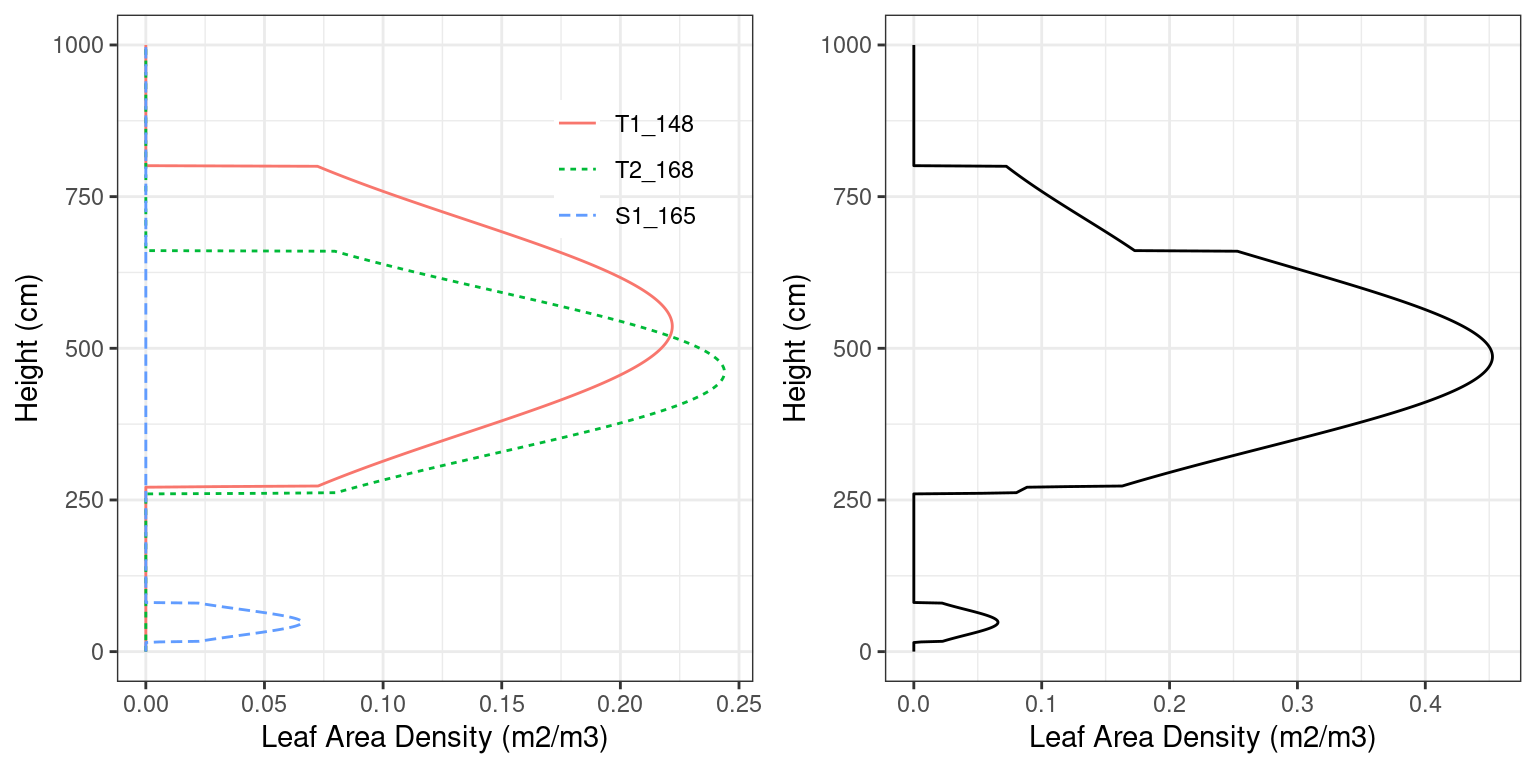
Figure 2.4: Leaf area density distribution of woody vegetation in a forest stand. The left panel shows the distribution for each plant cohort separately, whereas the right panel shows the overall density distribution.

The leaf area density profile determines the light extinction rates through the forest canopy. The same truncated Gaussian distribution is used to distribute leaf and small branch biomass along the vertical dimension.

When present, we can include herbaceous vegetation (i.e. \(LAI_{herb}\)) in the leaf area density profile. Its vertical distribution is also assumed to follow a truncated Gaussian function:

Figure 2.5: Leaf area density distribution in a forest stand, including the herbaceous layer. The left panel shows the distribution for each plant cohort separately, whereas the right panel shows the overall density distribution.

2.4.7 Vertical root distribution

Roots can be distinguished functionally into two different organs: coarse roots are responsible for mechanical support and transport of water and nutrients towards the stem, whereas fine roots are responsible for absorbing water and nutrients.

Analogously to the aboveground vegetation parameters, inputs describing depths corresponding to 50% and 95% of fine roots (\(Z_{50,i}\) and \(Z_{95,i}\)) are used to completely specify the distribution of roots across soil layers. The root system of each plant cohort \(i\) is described using \(FRP_{i,s}\), the proportion of fine roots (with respect to the whole plant) in each soil layer \(s\). \(FRP_{i,s}\) values are normally defined using the linear dose response model (Schenk & Jackson 2002; Collins & Bras 2007): \[\begin{eqnarray} FRP_{i,s} &=& Y_i(Z_s) - Y_i(Z_{s-1}) \\ Y_i(z) &=& \frac{1}{1+(z/Z_{50,i})^{c_i}} \end{eqnarray}\] where \(Y_i(z)\) is the cumulative fraction of fine root mass located between surface and depth \(z\); \(Z_{50,i}\) is the depth (in mm) above which 50% of the root mass is located; and \(c_i\) is a shape parameter related to \(Z_{50,i}\) and \(Z_{95,i}\) as \(c_i = 2.94 / \ln(Z_{50,i} / Z_{95,i})\).

The linear dose response model is quite flexible with respect to fine root distribution (see function root_ldrDistribution()). The following figure shows the fine root distribution profile of the same cohorts as in fig. 2.4 (see vprofile_rootDistribution()):

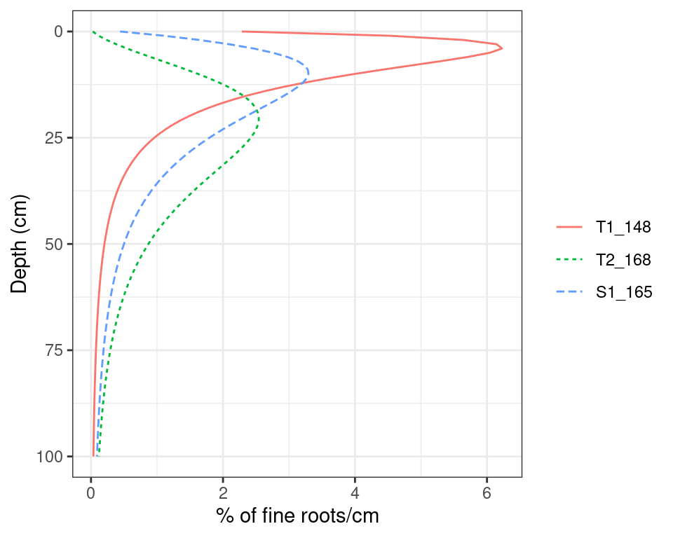
Figure 2.6: Examples of root density profile according to the linear dose response model.

The actual input to simulation functions spwb(), growth() and alike, describes fine root distribution using the matrix of \(FRP_{i,s}\) values - not \(Z_{50,i}\) and \(Z_{95,i}\) -, which means that the proportions of fine roots can be modified manually or be defined by another model. In fact, medfate also allows calculating \(FRP_{i,s}\) values assuming a conic distribution of fine roots (see root_conicDistribution()).

2.4.8 Optional variables in forest objects

The structure presented above for forest objects corresponds to the required data elements. A forest object can contain additional information when this is available. In particular, data frames treeData and shrubData can contain additional columns:

• LAI: Leaf area index (\(m^2 \cdot m^{-2}\)), corresponding to \(LAI^{live}\), avoiding the use of allometric relationships for leaf biomass in water balance simulations.
• FoliarBiomass: Standing dry biomass of leaves (\(kg \cdot m^{-2}\)), which together with \(SLA\) will be used to estimate \(LAI^{live}\), avoiding the use of allometric relationships for leaf biomass in water balance simulations.
• FuelLoading: Fine fuel loading (\(kg \cdot m^{-2}\)), to avoid its calculation from allometric relationships.
• CrownRatio: The ratio between crown length and total height (between 0 and 1), avoiding the use of allometric relationships for crown ratio in water balance simulations.
• Z100: Depth (in \(mm\)) corresponding to 100% of fine roots (to specify a truncated root distribution).
• ObsID: A string identifying plant cohorts at the stage of forest sampling. Used to track the fate of particular plant cohorts through simulations.

2.4.9 Water pools and root horizontal distribution

By default, models in medfate assume that soil moisture under all plant cohorts is the same (i.e. water sources corresponding to vertical soil layers are shared among cohorts). Therefore, it neglects spatial variation in soil moisture, against moisture variation patterns observed in mixed stands (Schume et al. 2004). However, variations in soil moisture beneath plant cohorts (and, implicitly, horizontal variation of soil moisture) can also be simulated if required by the user (see parameter rhizosphereOverlap in 2.6). This involves considering that a given plant cohort will perform water uptake from the water pool surrounding its roots, whereas it may not have access to the water beneath other plants. However, there can exist some degree of horizontal overlap between water pools exploited by different plants.

Considering water pools involves partitioning the stand area into fractions corresponding to the abundance of each plant cohort. More specifically, the model defines as many water pools as plant cohorts, with proportions defined by their LAI values: \[\begin{equation} f_{pool,i} = \frac{LAI^{live}_i}{LAI^{live}_{stand}} \end{equation}\] Models assume that the rhizosphere of each plant cohort occupies its own water pool but may extend into the water pools under other plant cohorts. In other words, the root systems of different cohorts may overlap horizontally. Moreover, the horizontal overlap of root systems will vary across soil layers. A given plant cohort \(i\) will have its roots in layer \(s\) partitioned among different water pools. We thus need to define \(fr_{i,s,j}\), the (horizontal) proportion of fine roots of cohort \(i\) in layer \(s\) of the water pool \(j\), with the restriction that: \[\begin{equation} \sum_{j}{fr_{i,s,j}} = 1 \,\, \forall i,s \end{equation}\]

A simplifying assumption is to force a complete independence of water pools, which is equal to say that \(fr_{i,s,j} = 1\) for \(i = j\) and \(fr_{i,s,j} = 0\) when \(i \neq j\) (this is the simplification adopted when using rhizosphereOverlap = "none"). In the general case of partial overlap (rhizosphereOverlap = "partial"), it is important to realize that proper estimation of \(fr_{i,s,j}\) is challenging when we do not have explicit plant coordinates, root lateral widths, etc. At this point, let us assume we have a reasonable estimate of \(Vol_{i}\), the soil volume explored by coarse roots of an individual of cohort \(i\). Assuming that the proportion of fine roots in each layer is proportional to the proportion of total soil volume explored by coarse roots that corresponds to the same layer we have that \(Vol_{i,s}\), the soil volume explored by coarse roots in layer \(s\) is: \[\begin{equation} Vol_{i,s} = FRP_{i,s}\cdot Vol_{i} \end{equation}\] In medfate, coarse roots are represented by axial and radial components. The length of axial component of a given layer (\(L_{axial, i, s}\)) is simply equivalent to its bottom depth, whereas the radial component (\(L_{radial, i, s}\)) is unknown. However, we can assume that the soil volume explored by coarse roots corresponds to a cylinder:
\[\begin{equation} Vol_{i,s} = \pi \cdot L_{radial,i,s}^2 \cdot L_{axial, i, s} \end{equation}\] and substituting the soil volume \(Vol_{i,s}\) in the equation above we can isolate \(L_{radial,i,s}\) (see function root_coarseRootLengthsFromVolume()). Once we have the radial component we can estimate the area (\(m^2\)) covered by coarse roots of an individual of the cohort in a given layer \(s\): \[\begin{equation} Area_{i,s} = \pi \cdot L_{radial,i,s}^2 \end{equation}\] We can then compare \(Area_{i,s}\) to the area of the water pool for an individual of cohort \(i\), which in \(m^2\) is: \[\begin{equation} AreaPool_{i} = 10000 \cdot f_{pool,i}/N_{i} \end{equation}\] If \(Area_{i,s} \leq AreaPool_{i}\), then the roots of the individual do not exceed the area of the pool, in other words \(fr_{i,s,i} = 1\) and \(fr_{i,s,j} = 0\) for all \(j \neq i\). If \(Area_{i,s} > AreaPool_{i}\) then the excess should be counted as overlap with the other pools. Assuming that plants are randomly distributed (i.e. no clumping) the probability of finding the pool of a cohort is equal to the proportion of its water pool (see function root_horizontalProportions()). All these calculations were done assuming \(Vol_{i}\) were known. Estimation of \(Vol_{i}\) depends on the complexity of the water balance model and is explained in A.4.6.

2.4.10 Functional traits and vegetation initialization

Besides the physical representation of vegetation, forest ecosystem models require information regarding plant functional traits, because this influences the outcome of physical, physiological and hydrological processes. In the following chapters, we will indicate for each simulated process its required plant functional parameters. A description of all parameters is provided in data frame SpParamsDefinition included in the package.

Normally, functional traits are described at the species level because infra-specific parameters are hard to get. Even at the species level, many functional (e.g. physiological) traits are hard to obtain, so in medfate we provide a default species parameter table for woody species found in Spain, with many of them occurring elsewhere in the Mediterranean Basin (SpParamsMED). User can modify this data frame to account for intra-specific trait variation (see function modifySpParams()).

The package provides functions spwbInput() and growthInput() that prepare the forest vegetation input for simulation functions spwb() and growth(), respectively (see 2.1.1). This initialization mostly consists in compiling the necessary functional traits from the species parameter table, following the \(SP_i\) attribute of woody plant cohorts. Some new model parameters are estimated from the initial ones, while taking into account the structural attributes of cohorts (an example of these derived quantities is stem conductance, which estimated from stem xylem conductivity, Huber value and plant height). Users can take the output of these initialization functions and replace parameter values for specific plant cohorts (see function modifyCohortParams()).

2.4.11 Update of structural variables during simulations

Vegetation characteristics stay constant during simulations using functions spwb() or pwb(), although the actual (unfolded) leaf area and dead leaf area may vary depending on leaf phenology.

In contrast, growth simulation requires updating the structure of vegetation, i.e. plant heights, tree diameters, tree density and shrub cover. Function growth() can modify any of the vegetation attributes. Finally, function fordyn() modifies not only structural variables of the initial cohorts but also involves the removal of dead (or cut) woody cohorts and recruitment of new woody cohorts during simulations.

2.5 Metereological input

Weather input data must include variables calculated at the daily scale. Weather data should be arranged in a data frame with days in rows and variables in columns.

Since it allows producing data frames with appropriate variable units and row/column names, we recommend meteorological input to be generated using package meteoland (De Cáceres et al. 2018), but other sources are possible.

2.5.1 Date format

Dates are needed in medfate to estimate parameters like solar declination or the day of the year (\(DOY\)). Dates can be specified in the input data frame either:

• As data frame row names (in string format year-month-day)
• As Date elements in a column called "dates".

2.5.2 Required weather variables

Some weather variables must be present always in the input data frame, whereas others are optional, meaning that the package can estimate them if missing. The following table indicates the symbols, units, definitions and the variable name in R of input weather variables that are always required:

Symbol	Units	R param	Description	Optional
\(T_{min}\)	\(^{\circ} \mathrm{C}\)	MinTemperature	Minimum temperature	No
\(T_{max}\)	\(^{\circ} \mathrm{C}\)	MaxTemperature	Maximum temperature	No
\(RH_{min}\)	%	MinRelativeHumidity	Minimum relative humidity	No
\(RH_{max}\)	%	MaxRelativeHumidity	Maximum relative humidity	No
\(P\)	\(L \cdot m^{-2} = mm\)	Precipitation	Precipitation (either rainfall or snow).	No
\(Rad\)	\(MJ \cdot m^{-2}\)	Radiation	Solar radiation after accounting for clouds	No

2.5.3 Optional weather variables

The following table lists the same attributes for input weather variables that are optional:

Symbol	Units	R param	Description	Optional
\(u\)	\(m \cdot s^{-1}\)	WindSpeed	Wind speed	Yes
\(R_{int}\)	\(mm \cdot h^{-1}\)	RainfallIntensity	Rainfall intensity	Yes
\(C_{atm}\)	\(ppm\)	CO2	Atmospheric (above-canopy) \(CO_2\) concentration	Yes
\(P_{atm}\)	\(kPa\)	Patm	Surface atmospheric pressure	Yes
\(P_{fire}\)	[0-1]	FireProbability	Probability of wildfire occurrence	Yes

Missing wind speed (\(u\)) and \(CO_2\) values will be replaced by defaults defined in control parameters. As an alternative to providing daily atmospheric \(CO_2\) concentration values, simulation functions allow the user to provide \(CO_2\) concentration values in annual time steps using a separate vector.

When missing, atmospheric pressure (\(P_{atm}\)) is also derived from elevation using an utility function available in meteoland.

Missing rainfall intensity (\(R_{int}\)) values will be estimated from the current month using function hydrology_rainfallIntensity() and the seasonality of rainfall intensity given in control parameters (see defaultRainfallIntensityPerMonth in 3.5.3).

2.5.4 Derived weather variables

While the weather variables listed in the tables above are provided as inputs, medfate derives other atmospheric variables from them, using also topographic information (see utility functions of the meteoland reference manual):

Symbol	Units	R param	Description
\(\rho_{air}\)	\(kg \cdot m^{-3}\)		Air density
\(e_{atm}\)	\(kPa\)		Atmospheric water vapor pressure
\(T_{mean}\)	\(^{\circ} \mathrm{C}\)	MeanTemperature	Mean daily temperature
\(PET\)	\(L \cdot m^{-2} = mm\)	PET	Potential evapotranspiration, calculated using Penman’s (1948) equation

2.6 Simulation control

Simulation control parameters are a list of global parameter values, initialized using function defaultControl(), that the user can modify to change the general behavior of simulation functions. Here is the set of global control parameters currently accepted in medfate:

names(defaultControl())

##   [1] "fillMissingRootParams"            "fillMissingSpParams"             
##   [3] "fillMissingWithGenusParams"       "verbose"                         
##   [5] "subdailyResults"                  "standResults"                    
##   [7] "soilResults"                      "snowResults"                     
##   [9] "plantResults"                     "plantWaterBalanceResults"        
##  [11] "labileCarbonBalanceResults"       "plantStructureResults"           
##  [13] "growthMortalityResults"           "leafResults"                     
##  [15] "temperatureResults"               "fireHazardResults"               
##  [17] "fireHazardStandardWind"           "fireHazardStandardDFMC"          
##  [19] "transpirationMode"                "soilFunctions"                   
##  [21] "VG_PTF"                           "ndailysteps"                     
##  [23] "max_nsubsteps_soil"               "defaultWindSpeed"                
##  [25] "defaultCO2"                       "defaultRainfallIntensityPerMonth"
##  [27] "leafPhenology"                    "bareSoilEvaporation"             
##  [29] "unlimitedSoilWater"               "interceptionMode"                
##  [31] "infiltrationMode"                 "infiltrationCorrection"          
##  [33] "soilDomains"                      "rhizosphereOverlap"              
##  [35] "unfoldingDD"                      "verticalLayerSize"               
##  [37] "windMeasurementHeight"            "segmentedXylemVulnerability"     
##  [39] "stemCavitationRecovery"           "leafCavitationRecovery"          
##  [41] "lfmcComponent"                    "hydraulicRedistributionFraction" 
##  [43] "nsubsteps_canopy"                 "taper"                           
##  [45] "multiLayerBalance"                "sapFluidityVariation"            
##  [47] "TPhase_gmin"                      "Q10_1_gmin"                      
##  [49] "Q10_2_gmin"                       "rootRadialConductance"           
##  [51] "averageFracRhizosphereResistance" "thermalCapacityLAI"              
##  [53] "boundaryLayerSize"                "cavitationRecoveryMaximumRate"   
##  [55] "sunlitShade"                      "numericParams"                   
##  [57] "leafCavitationEffects"            "stemCavitationEffects"           
##  [59] "stomatalSubmodel"                 "plantCapacitance"                
##  [61] "cavitationFlux"                   "soilDisconnection"               
##  [63] "leafCuticularTranspiration"       "stemCuticularTranspiration"      
##  [65] "C_SApoInit"                       "C_LApoInit"                      
##  [67] "k_SSym"                           "fractionLeafSymplasm"            
##  [69] "gs_NightFrac"                     "JarvisPAR"                       
##  [71] "fTRBToLeaf"                       "subdailyCarbonBalance"           
##  [73] "allowDessication"                 "allowStarvation"                 
##  [75] "sinkLimitation"                   "shrubDynamics"                   
##  [77] "herbDynamics"                     "allocationStrategy"              
##  [79] "phloemConductanceFactor"          "nonSugarConcentration"           
##  [81] "equilibriumOsmoticConcentration"  "minimumRelativeStarchForGrowth"  
##  [83] "constructionCosts"                "senescenceRates"                 
##  [85] "maximumRelativeGrowthRates"       "mortalityMode"                   
##  [87] "mortalityBaselineRate"            "mortalityRelativeSugarThreshold" 
##  [89] "mortalityRWCThreshold"            "recrTreeDBH"                     
##  [91] "recrTreeDensity"                  "ingrowthTreeDBH"                 
##  [93] "ingrowthTreeDensity"              "allowSeedBankDynamics"           
##  [95] "allowRecruitment"                 "allowResprouting"                
##  [97] "recruitmentMode"                  "removeEmptyCohorts"              
##  [99] "minimumTreeCohortDensity"         "minimumShrubCohortCover"         
## [101] "dynamicallyMergeCohorts"          "keepCohortsWithObsID"            
## [103] "seedRain"                         "seedProductionTreeHeight"        
## [105] "seedProductionShrubHeight"        "probRecr"                        
## [107] "minTempRecr"                      "minMoistureRecr"                 
## [109] "minFPARRecr"                      "recrTreeHeight"                  
## [111] "recrShrubCover"                   "recrShrubHeight"                 
## [113] "recrTreeZ50"                      "recrShrubZ50"                    
## [115] "recrTreeZ95"                      "recrShrubZ95"

Control parameters are employed when initializing vegetation inputs and state variables using functions spwbInput() and growthInput(), since they are needed also to make decisions at the point of initialization. Control parameters are also stored in the result of these functions, so the user does not need to specify again control parameters when calling simulation functions such as spwb() or growth(). Function fordyn() is different than the other simulation functions, because the list control parameters is directly passed to the function (see 2.1.1).

Even if the list of control parameters is long, not all control parameters are relevant to all simulation functions (this will be indicated in the following chapters), and most of them should not be altered from their default values. However, there are a set of parameters that are worth learning:

• verbose [=TRUE]: Whether extra console output is desired during simulations.
• transpirationMode [="Granier"] is an important control parameter, because it allows the user to switch between the basic (i.e. "Granier") and advanced (i.e., either "Sperry" or "Sureau") water balance models, corresponding to chapters 3 and 7, respectively.
• soilDomains [="buckets"] is an important control parameter, because it specifies how water moves between soil layers. Accepted values are "buckets" (for multi-bucket model), "single" (for single-domain Richards model) and "dual" (for dual-permeability model). See 5.7.
• rhizosphereOverlap [="total"] is also a relevant parameter, since changing its default value allows considering that plants extract soil water from partially or totally unrelated water pools, as explained in 2.4.9.

Some parameters are only relevant for parameter estimation at the stage of initialization:

• fillMissingRootParams [= TRUE]: Boolean flag to indicate that initialization functions should provide estimates for Z50 and Z95 if these are lacking in the forest data. Note that if fillMissingRootParams is set to FALSE then simulations may fail if the user does not provide values for Z50 and Z95 in tree or shrub data.
• fillMissingSpParams [=TRUE]: Boolean flag to indicate that initialization functions should provide estimates for functional parameters if these are lacking in the species parameter table SpParams. Note that if fillMissingSpParams is set to FALSE then simulations may fail if the user does not provide values for required parameters.
• fillMissingWithGenusParams [=TRUE]: Boolean flag to indicate that initializing functions should provide estimates from genus value, if species-level values are missing in the species parameter table SpParams but genus-level ones are not.

Bibliography

Carsel, R.F. & Parrish, R.S. (1988). Developing joint probability distributions of soil water retention characteristics. Water Resources Research, 24, 755–769.

Collins, D.B.G. & Bras, R.L. (2007). Plant rooting strategies in water-limited ecosystems. Water Resources Research, 43, W06407.

De Cáceres, M., Martin-StPaul, N., Turco, M., Cabon, A. & Granda, V. (2018). Estimating daily meteorological data and downscaling climate models over landscapes. Environmental Modelling & Software, 108, 186–196.

Genuchten, M.V. (1980). A closed-form equation for predicting the hydraulic conductivity of unsaturated soils. Soil science society of America journal, 44, 892–898.

Rahimi, A.A., Sepaskhah, A.R. & Ahmadi, S.H. (2011). Evaluation of different methods for the prediction of saturated hydraulic conductivity in tilled and untilled soils. Archives of Agronomy and Soil Science, 57, 899–914.

Ruffault, J., Martin-StPaul, N.K., Rambal, S. & Mouillot, F. (2013). Differential regional responses in drought length, intensity and timing to recent climate changes in a Mediterranean forested ecosystem. Climatic Change, 117, 103–117.

Saxton, K.E. & Rawls, W.J. (2006). Soil water characteristic estimates by texture and organic matter for hydrologic solutions. Soil Science Society of America Journal, 70, 1569.

Saxton, K.E., Rawls, W.J., Romberger, J.S. & Papendick, R.I. (1986). Estimating generalized soil-water characteristics from texture. Soil Science Society of America Journal, 50, 1031–1036.

Schenk, H.J. & Jackson, R.B. (2002). Rooting depths, lateral root spreads and below-ground/above-ground allometries of plants in water-limited ecosystems. Journal of Ecology, 90, 480–494.

Schume, H., Jost, G. & Hager, H. (2004). Soil water depletion and recharge patterns in mixed and pure forest stands of European beech and Norway spruce. Journal of Hydrology, 289, 258–274.

Stolf, R., Thurler, Á., Oliveira, O., Bacchi, S. & Reichardt, K. (2011). Method to estimate soil macroporosity and microporosity based on sand content and bulk density. Revista Brasileira de Ciencias do Solo, 35, 447–459.

Tóth, B., Weynants, M., Nemes, A., Makó, A., Bilas, G. & Tóth, G. (2015). New generation of hydraulic pedotransfer functions for Europe. European Journal of Soil Science, 66, 226–238.