Chapter 11 Leaf/canopy photosynthesis

In chapter 10 we introduced the necessary concepts of steady-state plant hydraulics to define the hydraulic supply function for the soil-plant continuum. The supply function specifies the flow rate, as per leaf area, for values of leaf water potential and given a soil moisture status. In the first section of this chapter we describe leaf photosynthesis functions, which define leaf gas exchange, photosynthesis and energy balance for values of leaf water potential. This requires knowing wind, water vapor and temperature conditions of the air surrounding leaves (section 13.1.3), the short-wave radiation absorbed by leaf elements (section 9.1.3) and the leaf long-wave radiation balance (section 9.2). In the second section of this chapter we discuss how to upscale photosynthesis values to the crown level.

11.1 Leaf energy balance, gas exchange and photosynthesis

The supply function specifies the transpiration flow rate $E$ for values of leaf water potential $\Psi_{leaf}$. If we know air temperature, water vapor pressure and the light conditions in which leaves are, we can translate the supply function into a leaf photosynthesis function (Sperry et al. 2017). In a nutshell, $E$ from the supply function is first used to calculate leaf temperature from an evaluation of the leaf energy balance. The diffusive conductances of the leaf to $H_2O$ and $CO_{2}$ are obtained from water supply and leaf water vapor deficit. Finally, the gross/net assimilation rate is then obtained from the diffusive conductance and a modelled curve between assimilation and leaf internal $CO_{2}$ concentration. The following subsections detail each of these steps separately.

11.1.1 Leaf temperature

Leaf temperature ($T_{leaf}$; in $^\circ C$) can be calculated for any given flow rate $E$ using an energy balance equation (Campbell & Norman 1998): \[\begin{equation} T_{leaf} = T_{air}+\frac{\Phi_{SWR}^{leaf} + L_{net}^{leaf}-\lambda_v(T_{air})\cdot E_{two-sided}}{C_p\cdot(g_r+g_{Ha})} \tag{11.1} \end{equation}\] where $\Phi_{SWR}^{leaf}$ (in $W \cdot m^{-2}$) is the instantaneous shortwave radiation absorbed per leaf area unit, $L_{net}^{leaf}$ is the instantaneous net long-wave radiation per leaf area unit, $E_{two-sided}$ is the flow rate $E$ converted to $mol \cdot s^{-1} \cdot m^{-2}$ per two-sided leaf area basis, $\epsilon$ is longwave radiation emissivity (0.97), $\sigma$ is the Stephan-Boltzman constant, $T_{air}$ is the temperature of the air surrounding the leaf (in $^\circ C$), $C_p$ = 29.3 $J \cdot mol^{-1} \cdot ºC^{-1}$ is the specific heat capacity of dry air at constant pressure and $\lambda_v(T_{air})$ is the latent heat of vaporization (in $J \cdot mol^{-1}$) corresponding to $T_{air}$ (see utility functions in the meteoland reference manual). If canopy energy balance is performed assuming a single canopy layer $T_{air}$ corresponds to $T_{can}$, the whole-canopy air temperature resulting from the energy balance of the previous step (see section 13.1.3). If a multi-layer canopy energy balance is used, $T_{air}$ corresponds to $T_{air,j}$, the air temperature of the canopy layer $j$ that contains the leaf. Finally, $g_r$ and $g_{Ha}$ are the radiative and heat conductance values (in $mol \cdot m^{-2} \cdot s^{-1}$), respectively (Campbell & Norman 1998): \[\begin{eqnarray} g_r &=& \frac{4\cdot \epsilon \cdot \sigma \cdot (T_{air}+273.15)^3}{C_p} \\ g_{Ha} &=& 0.189 \cdot (u_{leaf}/d)^{0.5} \tag{11.2} \end{eqnarray}\] where $u_{leaf}$ is the leaf-level wind speed (in $m \cdot s^{-1}$) and $d$ is 0.72 times the leaf width (species parameter LeafWidth in $cm$). As before, $u_{leaf}$ corresponds to $u_j$, the wind-speed at the canopy layer $j$ where the leaf is located (see 23.2).

By inspecting eq. (11.1), we can conclude that transpiration flow decreases leaf temperature, whereas radiation increases it and wind speed makes it more similar to the temperature of the surrounding air. The following figures illustrate the effect of varying wind speed and flow rate on $T_{leaf}$ for two contrasted leaf widths (see function biophysics_leafTemperature):

## Package 'meteoland' [ver. 2.2.1]

$Values of $T_{leaf}$ for two leaf widths and varying values of wind speed and flow rate, calculated for 24ºC air temperature and 740 $W \cdot m^{-2}$ instantaneous absorbed radiation (including SWR and LWR).$

Figure 11.1: Values of $T_{leaf}$ for two leaf widths and varying values of wind speed and flow rate, calculated for 24ºC air temperature and 740 $W \cdot m^{-2}$ instantaneous absorbed radiation (including SWR and LWR).

Let us now fix wind speed at the leaf leavel to $u_{leaf} = 2$ m/s. The application of the above equations to the $E(\Psi_{leaf})$ curves corresponding to the complete hydraulic network (10.4.5) yields the following $T_{leaf}(\Psi_{leaf})$ curves:

Examples of leaf temperature functions for a hydraulic network, corresponding to fig. 10.15 and for different soil textures. Left/right panel shows values for uncavitated/cavitated supply functions.

Figure 11.2: Examples of leaf temperature functions for a hydraulic network, corresponding to fig. 10.15 and for different soil textures. Left/right panel shows values for uncavitated/cavitated supply functions.

11.1.2 Leaf vapor pressure deficit

Vapor pressure deficit in the leaf ($VPD_{leaf}$, in kPa) is calculated as: \[\begin{equation} VPD_{leaf} = e_{leaf} - e_{air} \end{equation}\] Where $e_{air}$ is the water vapor pressure of the air surrounding the leaf (but beyond the leaf boundary layer) and $e_{leaf}$ is the leaf vapor pressure, which can be calculated from leaf temperature ($T_{leaf}$) and leaf water potential ($\Psi_{leaf}$): \[\begin{equation} e_{leaf} = e_{sat}(T_{leaf}) \cdot \exp\left\{\frac{2.17 \cdot \Psi_{leaf}}{T_{leaf}+273.15}\right\} \tag{11.3} \end{equation}\] where $e_{sat}(T)$ is a function giving the saturated vapor pressure for temperature $T$ (see utility functions of the meteoland reference manual). If a single-canopy energy balance is considered, the water vapor pressure of the air surrounding the leaf is taken as the average atmospheric water vapor pressure of the day, i.e. $e_{air} = e_{atm}$. When a multi-layer canopy energy balance is simulated, $e_{air}$ will correspond to the water vapor pressure $e_{air,j}$ of the canopy layer $j$ where the leaf is located.

Since $e_{leaf}$ decreases when leaf temperature decreases in eq. (11.3), increasing transpiration decreases leaf VPD as a result of decreasing leaf temperature. To illustrate this effect, let us assume the following values of relative humidity, yielding a $e_{air} = e_{atm} =1.91\, kPa$:

RHmin = 60
RHmax = 75
VPatm = meteoland::utils_averageDailyVP(Tmin, Tmax, RHmin, RHmax)
VPatm

## [1] 1.912181

The application of the above equation to the $T_{leaf}(\Psi_{leaf})$ curves of fig. 11.2 yields the following $VPD_{leaf}(\Psi_{leaf})$ curves:

$Examples of leaf vapour pressure deficit ($VPD_{leaf}$) functions for a hydraulic network, corresponding to fig. 10.15 and for different soil textures. Left/right panel shows values for uncavitated/cavitated supply functions.$

Figure 11.3: Examples of leaf vapour pressure deficit ($VPD_{leaf}$) functions for a hydraulic network, corresponding to fig. 10.15 and for different soil textures. Left/right panel shows values for uncavitated/cavitated supply functions.

Note that the VPD decreasing curves do not start at the same $VPD_{leaf}$ value despite corresponding to the same $T_{leaf}$ value, because of the effect of $\Psi_{leaf}$ on $e_{leaf}$ in eq. (11.3).

11.1.3 Leaf gas exchange

Leaf diffusive conductance to water vapor ($g_{w}$; in $mol\, H_2O \cdot s^{-1} \cdot m^{-2}$) and to carbon dioxide ($g_{c}$; in $mol\,CO_{2} \cdot s^{-1} \cdot m^{-2}$) are obtained for each value of transpiration flow $E$ (here expressed in $mol\, H_2O \cdot s^{-1} \cdot m^{-2}$) and $VPD_{leaf}$ using: \[\begin{eqnarray} g_{w} &=& E \cdot \frac{P_{atm}}{VPD_{leaf}}\\ g_{c} &=& g_{w}/1.6 \end{eqnarray}\] Diffusive conductance to water vapour is assumed to be result of stomatal ($g_{sw}$) and boundary layer ($g_{bw}$) conductances (both in $mol\, H_2O \cdot s^{-1} \cdot m^{-2}$). If we estimate $g_{bw}$ using: \[\begin{equation} g_{bw} = 0.397 \cdot (u_{leaf}/d)^{0.5} \end{equation}\] then, stomatal conductance is: \[\begin{equation} g_{sw}^{-1} = g_{w}^{-1} - g_{bw}^{-1} \end{equation}\] Ensuring here that $g_{w} \leq g_{bw}$ so that $g_{w}^{-1} \geq g_{bw}^{-1}$. The application of equations for $g_{w}$, $g_{bw}$ and $g_{sw}$ to the $VPD_{leaf}(\Psi_{leaf})$ curves yields the following stomatal conductance $g_{sw}(\Psi_{leaf})$ curves:

$Examples of stomatal conductance to water vapour ($g_{sw}$) functions for a hydraulic network, corresponding to fig. 10.15 and for different soil textures. Left/right panel shows values for uncavitated/cavitated supply functions. Minimum and maximum conductance values ($g_{sw,\min} = 0.0045$ and $g_{sw,\max} = 0.3$) are indicated using dashed lines.$

Figure 11.4: Examples of stomatal conductance to water vapour ($g_{sw}$) functions for a hydraulic network, corresponding to fig. 10.15 and for different soil textures. Left/right panel shows values for uncavitated/cavitated supply functions. Minimum and maximum conductance values ($g_{sw,\min} = 0.0045$ and $g_{sw,\max} = 0.3$) are indicated using dashed lines.

In the previous figure we have indicated the thresholds of $g_{sw,\min}$ and $g_{sw,\max}$, the species-specific minimum and maximum water vapour conductances (i.e. conductances when stomata are fully closed and fully open, respectively; see parameters Gswmin and Gswmax in SpParamsMED). $g_{sw}$ cannot exceed $g_{sw,\max}$ so that some flow rates may not be possible (see stomatal regulation below). However, $g_{sw,\max}$ should quickly become non-limiting as soil dries (i.e. reducing $E$) or $VPD_{leaf}$ increases (Sperry et al. 2017).

11.1.4 Leaf photosynthesis

Rubisco-limited photosynthesis rate $A_c$ (in $\mu mol\, CO_2 \cdot s^{-1} \cdot m^{-2}$) is modelled using (Collatz et al. 1991; Medlyn et al. 2002): \[\begin{equation} A_c=\frac{V_{max}\cdot (C_i- \Gamma*)}{C_i+K_c \cdot (1+ O_a/K_o)} \tag{11.4} \end{equation}\] where $V_{max}$ is Rubisco’s maximum carboxylation rate (in $\mu mol\, CO_2 \cdot s^{-1} \cdot m^{-2}$), $C_i$ is the internal carbon dioxide concentration (in $\mu mol \cdot mol^{-1}$), $\Gamma*$ is the compensation point (in $\mu mol \cdot mol^{-1}$), $K_c$ (in $\mu mol \cdot mol^{-1}$) and $K_o$ (in $mmol \cdot mol^{-1}$) are Michaelis-Menten constants for carboxylation and oxygenation, respectively, and $O_a$ is the atmospheric oxygen concentration (i.e. 209 $mmol \cdot mol^{-1}$). $\Gamma*$, $K_c$ and $K_o$ depend on leaf temperature ($T_{leaf}$, in $^\circ C$) (Bernacchi et al. 2001): \[\begin{eqnarray} \Gamma* &=& 42.75\cdot e^{\frac{37830\cdot (T_{leaf}-25)}{298\cdot R \cdot (T_{leaf}-273)}}\\ K_c &=& 404.9\cdot e^{\frac{79430\cdot (T_{leaf}-25)}{298\cdot R \cdot (T_{leaf}-273)}}\\ K_o &=& 278.4\cdot e^{\frac{36380\cdot (T_{leaf}-25)}{298\cdot R \cdot (T_{leaf}-273)}} \end{eqnarray}\] Electron transport-limited photosynthesis $A_e$ (in $\mu mol\, CO_2 \cdot s^{-1} \cdot m^{-2}$) was obtained from Medlyn et al. (2002): \[\begin{eqnarray} A_e &=& \frac{J}{4}\cdot \frac{C_i-\Gamma*}{C_i+2\cdot \Gamma*} \\ J &=& \frac{(\alpha\cdot Q^{leaf}_{PAR} + J_{max})-\sqrt{(\alpha\cdot Q^{leaf}_{PAR} + J_{max})^2-4.0\cdot c \cdot \alpha \cdot Q^{leaf}_{PAR} \cdot J_{max}}}{2\cdot c} \end{eqnarray}\] where $\alpha = 0.3\,mol \, e \cdot mol\,photon^{-1}$ is the quantum yield of electron transport, $Q^{leaf}_{PAR}$ is the absorbed PAR photon flux density per leaf area ($\mu mol\,photon \cdot m^{-2} \cdot s^{-1}$), which is calculated from absorbed PAR per leaf area ($\Phi^{leaf}_{PAR}$; in $W \cdot m^{-2}$): \[\begin{equation} Q^{leaf}_{PAR} = \Phi^{leaf}_{PAR}\cdot 546 \cdot 0.836\cdot 10^{-2} \tag{11.5} \end{equation}\] where $546$ is the wavelength in $nm$. $J_{max}$ and $J$ are the maximum and actual rate of electron transport (both in $\mu mol\,e \cdot m^{-2} \cdot s^{-1}$) and $c=0.9$ defines the curvature of the light-response curve. The gross assimilation rate $A$ at a given $C_i$ is the minimum of $A_e$ and $A_c$. To obtain a smooth $A$-vs-$C_i$ curve we used (Collatz et al. 1991): \[\begin{equation} A = \frac{(A_c+A_e)-\sqrt{(A_c+A_e)^2-4.0\cdot c'\cdot A_e\cdot A_c}}{2\cdot c'} \end{equation}\] where $c'=0.98$ is a curvature factor. The temperature dependence of $J_{max}$ and $V_{max}$ relative to 25ºC (i.e., relative to input parameters $J_{max,298}$ and $V_{max,298}$) is modelled using Leuning (2002) (his eq. 1 with parameters from his Table 2). The internal $CO_2$ concentration, $C_i$, needs to be known to calculate $A$ using the previous equations. Sperry et al. (2016) use a second equation for $A$ which uses $g_{c}$, the diffusive conductance to $CO_2$ (which includes both the stomatal conductance and boundary layer conductance): \[\begin{equation} A = g_{c} \cdot (C_{air}-C_i) \end{equation}\] where $C_{air}$ is the $CO_{2}$ concentration (in $\mu mol \cdot mol^{-1}$) in the air surrounding the leaf (beyond the leaf boundary layer). If a single-layer canopy energy balance is used then $C_{air}=C_{atm}$, the atmospheric $CO_{2}$ concentration (see weather input and parameter in function defaultControl()), whereas if a multi-layer canopy energy balance is used $C_{air}$ corresponds to $C_{air,j}$, the $CO_2$ concentration in the canopy layer $j$ where the leaf occurs, analogously to $T_{air}$ and $e_{air}$. Combining the two equations for $A$ and finding the root of the resulting equation using Newton-Raphson method allows determining $C_i$ and therefore $A$. Thus, after defining PAR photon flux density, atmosphere $CO_{2}$ concentration and maximum rate parameters:

Q = 2000
Catm = 386
Vmax298 = 100
Jmax298 = 1.67*Vmax298

one can obtain the following $A(\Psi_{leaf})$ curves from $T_{leaf}(\Psi_{leaf})$ and $g_{sw}(\Psi_{leaf})$:

$Examples of gross photosynthesis ($A$) functions for a hydraulic network, corresponding to fig. 10.15 and for different soil textures. Left/right panel shows values for uncavitated/cavitated supply functions.$

Figure 11.5: Examples of gross photosynthesis ($A$) functions for a hydraulic network, corresponding to fig. 10.15 and for different soil textures. Left/right panel shows values for uncavitated/cavitated supply functions.

Finally, leaf net photosynthesis ($A_n$; i.e. accounting for autotrophic respiration) is calculated as: \[\begin{equation} A_n = A - 0.015 \cdot V_{max} \end{equation}\]

11.2 Crown/canopy photosynthesis

In the previous subsection we showed how to calculate photosynthesis at the leaf level, but gross or net assimilation needs to be up-scaled to the crown or canopy levels, while accounting for the variation of leaf photosynthetic conditions across canopies. In this section, we briefly describe different alternatives for canopy/crown photosynthesis and justify our modelling choice.

11.2.1 Multi-layer canopy photosynthesis model

Ideally, crown or canopy photosynthesis requires repeating the calculations of leaf temperature, leaf VPD, leaf gas conductance and photosynthesis for every leaf. Multi-layer canopy models, however, divide the canopy into vertical layers and determine photosynthesis for each one (and each plant species or plant cohort, if required). Multi-layer models can account for the fact that environmental variables usually vary across the crown, including direct/diffuse absorbed radiation, air temperature, wind speed, water vapor pressure and $CO_2$ concentration. The amount of SWR and PAR absorbed per unit of leaf area at each canopy layer was shown in fig. 9.2.

Not only environmental factors, but leaves themselves may be different across canopy layers. Importantly, it is generally accepted that sunlit and shade leaves need to be treated separately (De Pury & Farquhar 1997). Separating the two kinds of leaves acknowledges that they operate at different parts of the light-saturation curve. Following De Pury & Farquhar (1997), we further assume that maximum carboxylation and electron transport rates are highest for leaves at the top of the canopy and there is a exponential decrease from there towards the bottom, where maximum rates are 50% of those at the top: \[\begin{eqnarray} V_{max,298,i,j} &=& V_{max,298,i}\cdot \exp(-0.713\cdot \sum_{h>i}{LAI^{\phi}_{h,j}}/LAI_i^{\phi}) \\ J_{max,298,i,j} &=& J_{max,298,i}\cdot \exp(-0.713\cdot \sum_{h>i}{LAI^{\phi}_{h,j}}/LAI_i^{\phi}) \end{eqnarray}\] where $LAI^{\phi}_{i,j}$ is the LAI value of the plant cohort $i$ at a given canopy layer $j$ and $LAI_i^{\phi}$ is the expanded LAI of the plant cohort. The following figure illustrate this decrease for the single-species canopy example of section 9.1.3:

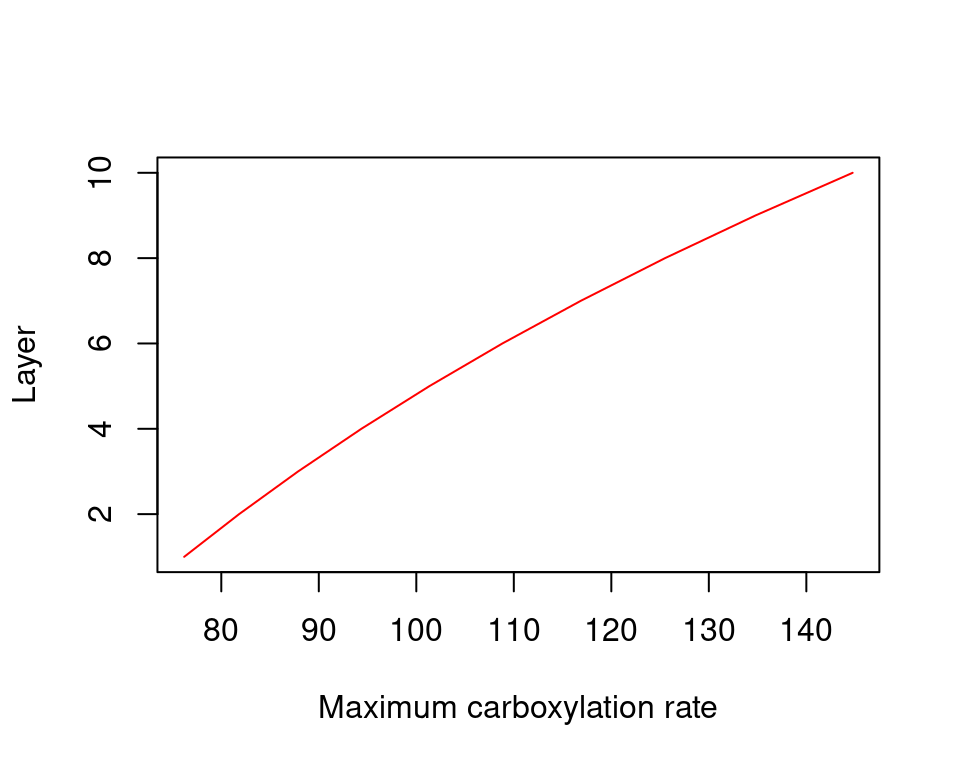
Figure 11.6: Decrease of Rubisco maximum carboxilation rate across the canopy

In a multi-layer canopy photosynthesis model, gross and net photosynthesis values (i.e. $A$ and $An$) are determined for sunlit and shade leaves of each cohort in each canopy layer. Then, sunlit and shade photosynthesis values should be averaged across the crown for each plant cohort. Assuming that $\Psi_{leaf}$ is equal for all leaves across the crown, the function $A(\Psi_{leaf})$ would be obtained for each plant cohort.

11.2.2 Big-leaf canopy photosynthesis model

Multi-layer canopy photosynthesis models allow evaluating leaf conditions, stomatal conductance and photosynthesis for different points of the canopy. However, this comes at high computational cost. For this reason, many models implement what is called the big-leaf approximation. Assuming that wind speed, temperature, water vapor pressure and $CO_2$ concentration are similar for all leaves and that the distribution of photosynthetic capacity between leaves is in proportion to the profile of absorbed irradiance then the equation describing leaf photosynthesis will also represent canopy photosynthesis (Sellers et al. 1992).

11.2.3 Sun-shade canopy photosynthesis model

An alternative between multi-layer and big-leaf canopy photosynthesis models is to collapse variation of photosynthetic conditions into two leaf classes: sunlit and shade leaves. While big-leaf canopy models are known to be unaccurate under some situations, sun-shade canopy models (De Pury & Farquhar 1997) provide estimates that are close to multiple layer models (Hikosaka et al. 2016). The sun-shade canopy photosynthesis model was adopted here. Assuming that wind speed, temperature, water vapor pressure and and $CO_2$ concentration are similar for all leaves, sun-shade models involve the following steps:

Aggregate the leaf area of sunlit/shade leaves across layers: \[\begin{eqnarray} LAI^{sunlit}_{i} &=& \sum_{j=1}^{l}{LAI^{sunlit}_{i,j}} \\ LAI^{shade}_{i} &=& \sum_{j=1}^{l}{LAI^{shade}_{i,j}} \end{eqnarray}\] where $LAI^{sunlit}_{i,j}$ and $LAI^{shade}_{i,j}$ are the leaf area index of sunlit and shade leaves for cohort $i$ in canopy layer $j$, from eq. (9.1).
Average the SWR/PAR absorbed by leaves of each kind across layers. The average light absorbed by sunlit/shaded foliage of cohort $i$ per ground area unit is found using: \[\begin{eqnarray} \Phi^{sunlit}_{abs,i} &=& \frac{\sum_{j=1}^{l}{K^{sunlit}_{abs,i,j}}}{LAI^{sunlit}_{i}} \\ \Phi^{shade}_{abs,i} &=& \frac{\sum_{j=1}^{l}{K^{shade}_{abs,i,j}}}{LAI^{shade}_{i}} \end{eqnarray}\] where $K^{sunlit}_{abs,i,j}$ and $K^{shade}_{abs,i,j}$ are the light absorbed per ground area unit by sunlit/shade leaves of cohort $i$ at layer $j$ (see section 9.1.3). Analogous equations were already given for the net long-wave radiation balance of sunlit leaves ($L^{sunlit}_{net,i}$) and shade leaves ($L^{shade}_{net,i}$) in section 9.2.3.
Average the maximum carboxylation (respectively, electron transport) rates across layers, again separating sunlit and shade leaves: \[\begin{eqnarray} V^{sunlit}_{max,298,i} &=& \frac{\sum_{j=1}^{l}{V_{max,298,i,j} \cdot LAI^{sunlit}_{i,j}}}{LAI^{sunlit}_{i}} \\ V^{shade}_{max,298,i} &=& \frac{\sum_{j=1}^{l}{V_{max,298,i,j} \cdot LAI^{shade}_{i,j}}}{LAI^{shade}_{i}} \end{eqnarray}\]
Use $V^{sunlit}_{max,298,i}$ as $V_{max,298}$ in Leuning (2002) to obtain $V_{max}$ for eq. (11.4); $\Phi^{sunlit}_{SWR,i}$ as $\Phi^{leaf}_{SWR}$ and $L^{sunlit}_{net,i}$ as $L^{leaf}_{net}$ in eq. (11.1); and $\Phi^{sunlit}_{PAR,i}$ as $\Phi_{PAR}^{leaf}$ in eq. (11.5) to estimate sunlit leaf photosynthesis, which can be up-scaled to the crown level multiplying by $LAI^{sunlit}_{i}$. The same would be done for shade leaves. In a sun-shade canopy model one then calls the photosynthesis function twice (i.e. once for shade leaves and once for sunlit leaves) for each plant cohort $i$.

11.2.4 Comparison of big-leaf, sun-shade and multi-canopy photosynthesis models

The figure below provides the canopy photosynthesis functions obtained using the multi-layer canopy photosynthesis model (top), a sunshade canopy photosynthesis model (center) or a big-leaf photosynthesis model (bottom). These were generated using functions photo_multilayerPhotosynthesisFunction(), photo_sunshadePhotosynthesisFunction() and photo_leafPhotosynthesisFunction(), respectively, and assuming homogeneous wind, temperature and water vapor pressure through the canopy. Thus, only absorbed radiation varied across layers and leaf types. Note the coincidence between the multi-layer and the sun-shade models.

Whole-canopy photosynthesis functions obtained for a hydraulic network, corresponding to fig. 10.15 and different soil textures, using the multi-layer canopy photosynthesis model (top), a sunshade canopy photosynthesis model (center) or a big-leaf photosynthesis model (bottom). Left/right panel shows values for uncavitated/cavitated supply functions.

Figure 11.7: Whole-canopy photosynthesis functions obtained for a hydraulic network, corresponding to fig. 10.15 and different soil textures, using the multi-layer canopy photosynthesis model (top), a sunshade canopy photosynthesis model (center) or a big-leaf photosynthesis model (bottom). Left/right panel shows values for uncavitated/cavitated supply functions.

11.2.5 Within-canopy variation in environmental conditions

When presenting the sun-shade photosynthesis model, we assumed constant wind, temperature, water vapor pressure and $CO_2$ concentration values through the canopy. If a single-layer canopy energy balance is used, $CO_2$ concentration and vapor pressure are assumed equal to the atmosphere (i.e., $e_{air} = e_{atm}$ and $C_{air} = C_{atm}$), whereas air temperature is that of the canopy (i.e., $T_{air} = T_{can}$), but leaf-level wind speed ($u_{leaf}$) can still be different for different canopy layers. If a multi-layer canopy energy balance is used, all four environmental variables can differ between canopy layers (i.e. $T_{air,j}$, $e_{air,j}$, $C_{air,j}$ and $u_j$). In the sun-shade photosynthesis model, the question arises on how to determine layer $j$ for sunlit or shade leaves of a given cohort $i$. The choice is done by calculating the height corresponding to the mass center of sunlit leaves or shade leaves of each cohort $i$. The canopy layer $j$ where this mass center height is contained is chosen as the layer from which environmental conditions will be taken. For any given plant cohort $i$, sunlit leaves will take their environmental conditions from layers above (or equal to) those corresponding to shade leaves.

Bibliography

Bernacchi, C.J., Singsaas, E.L., Pimentel, C., Portis, A.R. & Long, S.P. (2001). Improved temperature response functions for models of Rubisco-limited photosynthesis. Plant, Cell and Environment, 24, 253–259.

Campbell, G.S. & Norman, J.M. (1998). An introduction to environmental biophysics. Springer-Verlag, New York.

Collatz, G.J., Ball, J.T., Grivet, C. & Berry, J.A. (1991). Physiological and environmental regulation of stomatal conductance, photosynthesis and transpiration: A model that includes a laminar boundary layer. Agricultural and Forest Meteorology, 54, 107–136.

De Pury, D.G.G. & Farquhar, G.D. (1997). Simple scaling of photosynthesis from leaves to canopies without the errors of big-leaf models. Plant, Cell and Environment, 20, 537–557.

Hikosaka, K., Kumagai, T. & Ito, A. (2016). Modeling Canopy Photosynthesis. pp. 239–268.

Leuning, R. (2002). Temperature dependence of two parameters in a photosynthesis model. Plant, Cell and Environment, 25, 1205–1210.

Medlyn, B.E., Loustau, D. & Delzon, S. (2002). Temperature response of parameters of a biochemically based model of photosynthesis. I. Seasonal changes in mature maritime pine (Pinus pinaster Ait.). Plant, Cell and Environment, 25, 1155–1165.

Sperry, J.S., Venturas, M.D., Anderegg, W.R.L., Mencuccini, M., Mackay, D.S., Wang, Y., et al. (2017). Predicting stomatal responses to the environment from the optimization of photosynthetic gain and hydraulic cost. Plant, Cell & Environment, 40, 816–830.

Sperry, J.S., Wang, Y., Wolfe, B.T., Mackay, D.S., Anderegg, W.R.L., Mcdowell, N.G., et al. (2016). Pragmatic hydraulic theory predicts stomatal responses to climatic water deficits. New Phytologist, 212, 577–589.