Chapter 17 Growth, senescence and mortality
17.1 Growth
17.1.1 Temperature and turgor sink limitations
Sink limitations due to temperature and turgor effects on growth are modelled following Cabon et al. (2020a) and Cabon et al. (2020b). These authors suggested equations to model sink limitations on cambium cell division and tracheid expansion, but we apply the same approach for simulating growth of leaves, sapwood and fine roots. Cell relative expansion rate (\(r_{cell}\)) is central to the approach by Cabon et al. and is defined as the relative time derivative of cell volume: \[\begin{equation} r_{cell} = \frac{dV}{Vdt} \end{equation}\] Cabon et al. (2020a) first suggested to model the dependence of \(r_{cell}\) on cell turgor using Lockhart’s equation: \[\begin{equation} r_{cell}(\Psi, \pi_0) = \phi_{max} \cdot (\Psi - \pi_0 - Y_{P}) \end{equation}\] where \(\Psi\) is the water potential, \(\pi_0\) is the osmotic water potential at full turgor, \(Y_P\) is the turgor yield threshold and \(\phi_{max}\) is the maximum cell wall extensibility. Later, Cabon et al. (2020b) suggested to account for both turgor and temperature limitations on \(r_{cell}\) using the following expanded equation: \[\begin{equation} r_{cell}(T, \Psi, \pi_0) = \phi_{max} \cdot (\Psi - \pi_0 - Y_{P}) \cdot \frac{f_{met}(T_K)}{f_{met}(288.15)} \cdot{f_{micro}(T, T_{thr})} \tag{17.1} \end{equation}\] where \(T\) is temperature, \(f_{met}(T_K)\) is a function modulating the effect of temperature \(T_K\) in Kelvin, on metabolic rate, and \(f_{micro}(T, T_{thr})\) is a sigmoidal function modulating the effect of temperature on microtubule stability, depending on a temperature threshold \(T_{thr}\). Function \(f_{met}(T_K)\) is defined as: \[\begin{equation} f_{met}(T_K) = \frac{T_K \cdot \exp \big\{ \frac{\Delta H_A}{R^n \cdot T_K}\big\}}{1 + \exp \big\{ \frac{\Delta S_D}{R^n} \cdot \left(1 - \frac{\Delta H_D}{\Delta S_D \cdot T_K} \right)\big\}} \end{equation}\] where \(R^n\) is the ideal gas constant, \(\Delta H_A = 87500\) the enthalpy of activation and \(\Delta H_D = 333000\) and \(\Delta S_D = 1090\) the enthalpy and entropy difference (respectively) between the catalytically active and inactive states of the enzymatic system).
In medfate, we assume a constant value of \(\pi_0 = -1\) in meristematic tissues, so that \(r_{cell}\) depends on \(\Psi\) and \(T\) only. Scaling from the cell to the tissue level is conducted by assuming that maximum cell-level expansion rates correspond to maximum tissue-level relative growth rates. Maximum cell-level expansion rates, \(r_{cell, max}\), are assumed to occur at \(T = 30^\circ C\) and \(\Psi = 0\). Other parameters for eq. (17.1) are set to \(\phi_{max} = 0.5\) (which becomes irrelevant), \(Y_{P} = 0.05\,MPa\) and \(T_{thr} = 5^\circ C\).
17.1.2 Leaf growth
Leaf area increment \(\Delta LA\) only occurs when phenological state is unfolding, and is defined as the minimum of three values expressing three corresponding constraints: \[\begin{equation} \Delta LA = \min( \Delta LA_{alloc}, \Delta LA_{source}, \Delta LA_{sink}) \end{equation}\] First, \(\Delta LA_{alloc}\) is the maximum leaf area increment allowed by the leaf area target set by the allocation rule, \(LA_{target}\), in comparison with current leaf area \(LA_{\phi}\): \[\begin{equation} \Delta LA_{alloc} = \max(LA_{target} - LA_{\phi},0) \end{equation}\] Remember that leaf area target is updated during bud formation (see 17.3.2).
Second, \(\Delta LA_{source}\) represents the leaf area increment expected given carbon source limitations and is calculated: \[\begin{equation} \Delta LA_{source} = \frac{ST_{sapwood}\cdot m_{gluc}\cdot V_{sapwood,leaf}}{1000 \cdot CC_{leaf} / SLA} \end{equation}\] where \(ST_{sapwood}\) is the current concentration of sapwood storage carbon (starch), \(V_{storage,sapwood}\) is the sapwood storage volume and \(m_{gluc}\) is glucose molar mass and the denominator contains the construction costs per leaf area unit, see eq. (16.4).
Finally, \(\Delta LA_{sink}\) represents the leaf area increment expected by taking into account the maximum leaf tissue growth rate relative to sapwood area (\(RGR_{leaf, max}\); in \(m^2 \cdot cm^{-2} \cdot day^{-1}\)), the percentage of the crown with active buds (\(PCAB\)) and the relative cell expansion rate given \(T_{day}\), \(\Psi_{symp,leaf}\) and \(\pi_{0,leaf}\): \[\begin{equation} \Delta LA_{sink} = SA \cdot (PCAB/100) \cdot RGR_{leaf, max} \cdot \frac{r_{cell}(T_{day}, \Psi_{symp,leaf})}{r_{cell,max}} \end{equation}\] where cell relative expansion rate is divided by the maximum relative cell expansion rate \(r_{cell,max}\), so that \(RGR_{leaf, max}\) is attained when sink conditions are optimal. The final expression of \(\Delta LA_{sink}\) reduces to a product of the maximum leaf area growth times two factors (for turgor and temperature) bounded between 0 and 1.
If previous drought or fire impacts had reduced the percentage of the crown with active buds (\(PCAB\)), this percentage is increased along with primary growth (i.e. with leaf growth), until it achieves 100%: \[\begin{equation} PCAB_{t+1} = \min(PCAB_{t} + RGR_{bud} \cdot \frac{\Delta LA}{LA_{target}}, 100) \end{equation}\] where \(RGR_{bud}\) is the growth rate of buds per unit per unit leaf area growth (\(m^2 \cdot m^{-2}\)).
17.1.3 Sapwood growth
Sapwood area increment \(\Delta SA\) can only occur if \(LA_{live}>0\). Newly assimilated carbon is preferentially allocated to leaves and fine roots whenever storage levels are low. \(\Delta SA\) is defined as the minimum of two values expressing source and sink constraints:
\[\begin{equation}
\Delta SA = \min(\Delta SA_{source}, \Delta SA_{sink})
\end{equation}\]
\(\Delta SA_{source}\) represents the sapwood area increment expected given carbon source limitations and is calculated using:
\[\begin{equation}
\Delta SA_{source} = \frac{\max(ST_{sapwood}-ST_{sapwood,growth},0)\cdot m_{gluc}\cdot V_{storage,sapwood}}{CC_{sapwood} \cdot (H + \sum_{s}{FRP_s \cdot L_s}) \cdot \rho_{wood}}
\end{equation}\]
where \(ST_{sapwood}\) is the current starch concentration, \(ST_{sapwood,growth}\) is the minimum starch concentration required for sapwood growth, \(V_{storage,sapwood}\) is the sapwood storage volume, \(m_{gluc}\) is glucose molar mass and the denominator contains the construction costs per sapwood area unit, see eq. (16.6). \(ST_{sapwood,growth}\) is related to the minimum relative starch concentration for growth (\(RSSG\)), which is specified via the species-specific parameter RSSG or the control parameter minimumRelativeStarchForGrowth. This parameter is important because it allows specifying to which extent a given plant species stops growth and saves carbon to ensure survival (e.g. shadow tolerant species), as opposed to a species strongly investing in growth to reach the top of the canopy and have access to high light levels (e.g. light-demanding species).
Assuming that the maximum relative sapwood growth rate (\(RGR_{cambium, max}\) or \(RGR_{sapwood, max}\)) corresponds to a maximum rate of daily ring area increase, we have that the daily increase in sapwood area according to sink limitations, \(\Delta SA_{sink}\), is defined as: \[\begin{equation} \Delta SA_{sink} = \pi \cdot DBH \cdot (PCAC/100) \cdot RGR_{cambium, max} \cdot \frac{r_{cell}(T_{day}, \Psi_{symp, stem})}{r_{cell,max}} \end{equation}\] for trees, and as: \[\begin{equation} \Delta SA_{sink} = SA \cdot (PCAC/100) \cdot RGR_{sapwood, max} \cdot \frac{r_{cell}(T_{day}, \Psi_{symp, stem})}{r_{cell,max}} \end{equation}\] for shrubs. Sapwood growth in trees is proportional to the cambium length (in \(cm\)), whereas in trees it is proportional to the current sapwood area (in \(cm^2\)). Hence, two different maximum relative growth rates are defined for trees (\(RGR_{cambium, max}\)) and shrubs (\(RGR_{sapwood, max}\)). In the above equations, \(PCAC\) is the percentage of active cambium cells, which is assumed to be controlled by the amount of foliage via the synthesis of growth hormones that then are transported through phloem. In practice, \(PCAC\) is estimated as: \[\begin{equation} PCAC = 100 \cdot \frac{LAI^{\phi}}{LAI^{NC}} \end{equation}\] where \(LAI_{\phi}\) is the currently expanded leaf area index and \(LAI_{NC}\) is the leaf area index assuming no competition with other plants. Since \(LAI_{\phi} = \phi \cdot LAI_{live}\) depends on the phenological status \(\phi\), the sapwood growth rate will depend on phenology. Moreover, since \(LAI_{live} \leq LAI_{NC}\), maximum growth rates will be achieved by cohorts lacking competition of taller cohorts and low self-competition. Since competition increases with forest development, the inclusion of \(PCAC\) ensures that sapwood area growth rates will decrease for forests of larger basal area.
17.1.4 Fine root growth
Fine root biomass increment is modelled for each soil layer separately, and is defined analogously to leaf area increment: \[\begin{equation} \Delta B_{fineroot} = \min( \Delta B_{fineroot,alloc}, \Delta B_{fineroot,source}, \Delta B_{fineroot,sink}) \end{equation}\] First, \(\Delta B_{fineroot,alloc}\) is the maximum fine root biomass increment allowed by the biomass target set by the allocation rule, \(B_{fineroot,target}\) (see 17.3.2), in comparison with current biomass, \(B_{fineroot}\): \[\begin{equation} \Delta B_{fineroot,alloc} = \max(B_{fineroot,target} - B_{fineroot},0) \end{equation}\]
Second, \(\Delta B_{fineroot,source}\) represents the biomass increment expected given the available storage carbon (starch): \[\begin{equation} \Delta B_{fineroot,source} = \frac{ST_{sapwood} \cdot m_{gluc}\cdot V_{storage,sapwood}}{CC_{fineroot}} \end{equation}\] where \(ST_{sapwood}\) is the current sapwood concentration of storage carbon, \(V_{storage,sapwood}\) is the sapwood storage volume, \(m_{gluc}\) is glucose molar mass and \(CC_{fineroot}\) is the construction costs per fine root biomass unit.
Finally, \(\Delta B_{fineroot,sink}\) represents the biomass increment expected by taking into account maximum tissue growth rate (\(RGR_{fineroot, max}\); in \(g\,dry \cdot g\,dry^{-1} \cdot day^{-1}\)) and the relative cell expansion rate given temperature (\(T_{day}\)) and water potential in the rhizosphere (\(\Psi_{rhizo,s}\)): \[\begin{equation} \Delta B_{fineroot,sink} = B_{fineroot} \cdot RGR_{fineroot, max} \cdot \frac{r_{cell}(T_{day}, \Psi_{rhizo,s})}{r_{cell,max}} \end{equation}\] cell relative expansion rate is divided by the maximum relative cell expansion rate so that \(RGR_{fineroot, max}\) is attained when sink conditions are optimal.
17.2 Senescence
17.2.1 Leaf aging and cavitation effects on leaves and buds
Leaf senescence can occur due to two processes: aging or hydraulic disconnection related to cavitation. Senescence due to advanced leaf age is assumed to be programmed (Ca+ accumulation?). In deciduous species all live leaf area turns to death leaf area when the phenology submodel indicates it (4.1.3). In evergreen species the proportion of leaf area that undergoes senescence each day is determined by the species-specific leaf duration parameter (\(LD\)): \[\begin{equation} p_{aging,leaf} = \frac{1}{365.25 \cdot LD} \end{equation}\] Leaf senescence can also occur as a consequence of hydraulic disconnection, as described in 6.2.3 and 14.5, for the basic or advanced water balance models, respectively. If the proportion of stem conductance loss has increased with respect to the preceeding day, the model determines \(LA_{cavitation}\), the maximum leaf area allowed according to the current level of cavitation, by estimating the cavitation-induced defoliation proportion and applying it to the maximum leaf area (\(LA_{target}\)). If \(LA_{cavitation} < LA\) then the corresponding proportion \(p_{cavitation, leaf}\) is estimated for senescence.
The maximum of \(p_{aging,leaf}\) and \(p_{cavitation, leaf}\) is finally applied to reduce \(LA\) and increase \(LA_{dead}\) correspondingly.
Xylem cavitation not only causes defoliation but also mortality of buds, which has the effect of slowing down post-drought leaf area recovery. The percentage of the crown with active buds (\(PCAB\)) is reduced whenever the proportion of conductance loss has increased with respect to the preceeding day:
\[\begin{equation} PCAB = \min(PCAB, 100 \cdot (1 - PLC_{stem})) \end{equation}\]
This reduction has an effect on subsequent leaf growth (see 17.1.2).
17.2.2 Sapwood senescence
The daily rate of sapwood senescence is specified via the species-specific parameter \(SR_{sapwood}\) or, when missing, via a control parameter. Prentice et al. (1993) assumed a constant annual rate of 4% for the conversion from sapwood to heartwood. Similarly, Sitch et al. (2003) assumed a sapwood annual turnover rate of 5% for all biomes. In our model, the proportion of sapwood area that is transformed into heartwood daily is estimated using: \[\begin{equation} p_{aging, sapwood} = \frac{SR_{sapwood}}{1+15\cdot e^{-0.01\cdot H}} \cdot \frac{\max(T_{day}-5,0)}{20} \end{equation}\] where \(SR_{sapwood}\) is a species-specific parameter, \(T_{day}\) is the average day temperature and 0.01 is a constant causing shorter plants to have slower senescence rates. It is important to mention that, while stem cavitation \(PLC_{stem}\) reduces the amount of functional sapwood in with respect to hydraulics (and therefore transpiration and photosynthesis), it does not increase the rate of sapwood senescence. Hence, when xylem embolism occurs air bubbles are formed within vessels but surrounding parenchymatic cells (as well as the storage carbon they contain) are assumed unaffected.
17.2.3 Fine root senescence
Aging is the only process leading to fine root senescence. The daily turnover proportion for fine roots (\(SR_{fineroot}\)) is assumed to correspond to a temperature of 25 ºC, is specified via species-specific parameters or the control parameters turnoverRates. Actual turnover proportion for a given soil layer (\(p_{aging,fineroot}\)) decreases linearly with soil temperature down to zero at 5 ºC:
\[\begin{equation}
p_{aging,fineroot} = SR_{fineroot} \cdot \frac{\max(T_{soil,s}-5,0)}{20}
\end{equation}\]
where \(T_{soil,s}\) is the temperature of soil layer \(s\). When \(SR_{fineroot}\) is missing from species parameter, a default control value for \(SR_{fineroot}\) is taken, which produces an annual 50% turnover of fine roots.
17.3 Update of plant traits and allocation targets
17.3.1 Plant traits
Multiple anatomic and physiological parameters are updated every day after applying changes in the size of leaf, sapwood and fine root compartments, which creates a feedback to those hydraulic and physiological processes simulated in the water balance submodel. Hence, the growth model allows emulating plant acclimation to environmental cues, mediated by growth and senescence of plant tissues.
First leaf area index (\(LAI_{\phi}\)) is updated from leaf area (\(LA_{\phi}\)) inverting eq. (16.2). The Huber value (\(H_v\), the sapwood area to leaf area ratio; in \(m^{2}\cdot m^{-2}\)) is affected by changes in \(LA_{live} = LA_{target}\) and sapwood area \(SA\): \[\begin{equation} H_v = \frac{SA/10000}{LA_{live}} \end{equation}\] Note that we specify \(LA_{live} = LA_{target}\) and not \(LA_{\phi}\) to avoid variations in Huber value due to leaf phenology. By definition, fine root biomass changes in each soil layer (\(B_{fineroot,s}\)) lead to updates in the proportion of fine roots in each layer (\(FRP_s\)): \[\begin{equation} FRP_s = \frac{B_{fineroot,s}}{\sum_{l}{B_{fineroot,l}}} \end{equation}\]
When we simulate growth with the advanced water balance model other parameters are subject to acclimation. Stem maximum conductance per leaf area unit (\(k_{stem, max}\); in \(mmol \cdot m^{-2}\cdot s^{-1} \cdot MPa^{-1}\)) is determined as a function of species-specific xylem conductivity (\(K_{xylem, max}\); in \(kg \cdot m^{-1} \cdot s^{-1} \cdot MPa^{-1}\)), leaf area, sapwood area and tree height (Christoffersen et al. 2016): \[\begin{equation} k_{stem, max} = \frac{1000}{0.018} \cdot \frac{K_{xylem, max} \cdot H_v}{(H/100)} \cdot \chi_{taper} \end{equation}\] where \(\chi_{taper}\) is a factor to account for taper of xylem conduit with height (Savage et al. 2010; Christoffersen et al. 2016), 0.018 is the molar weight of water (in \(kg\cdot mol^{-1}\)). Both an increase in \(SA\) or a decrease in \(LA_{live}\) (i.e. an increase in \(H_v\)) increase \(k_{stem, max}\) and, hence, alleviate drought effects (i.e. a lower decrease in water potential across the stem for the same flow). In contrast, an increase in plant height will decrease stem conductance and increase drought stress. Changes in stem maximum conductance has cascade effects on root maximum conductance. First, coarse root minimum resistance is defined as a fixed proportion of whole-plant minimum resistance, so an increase in stem maximum conductance will increase whole-plant conductance and coarse root conductance, \(k_{root,max}\).
Rhizosphere maximum conductance per leaf area unit in a given soil layer \(s\) (\(k_{rhizo, max, s}\); in \(mmol \cdot m^{-2}\cdot s^{-1} \cdot MPa^{-1}\)) depends on fine root biomass in this layer (\(B_{fineroot,s}\)) and on leaf area (i.e. \(LA_{live}\)). The equations regulating these relationships are modulated by several soil and species parameters, such as soil saturated hydraulic conductance, species-specific root length, root length density and density of fine roots.
The proportion of conductance loss due to cavitation (\(PLC_{stem}\)) is reduced whenever sapwood area growth occurs: \[\begin{equation} PLC_{stem, t+1} = \min(PLC_{stem,t} - \frac{\Delta SA}{SA},0) \end{equation}\] This allows a progressive increase in functional sapwood area.
17.3.2 Leaf area and fine root biomass targets
Leaf area target (\(LA_{live} = LA_{target}\)) is updated when phenological phase is bud formation. If the allocation strategy pursues a stable Huber value, the model tries to bring \(H_{v}\) close to an initial value \(H_{v,target}\), and the leaf area target is defined as: \[\begin{equation} LA_{live} = LA_{target} = \frac{SA}{10000 \cdot H_{v,target}} \end{equation}\] Note that the specification of \(LA_{target}\) will cause sapwood area increases to be followed by leaf area increases, as long as \(H_{v} > H_{v,target}\). On the contrary, if \(H_{v} < H_{v,target}\) then leaf area growth is inhibited and sapwood area growth will progressively increase \(H_{v}\). Fine root biomass target is set using: \[\begin{equation} B_{fineroot,target} = \frac{10^{4}\cdot LA_{target} \cdot RLR}{2.0 \cdot \sqrt{\frac{\pi \cdot SRL}{\rho_{fineroot}}}} \end{equation}\] where \(RLR\) is the root area to leaf area ratio, \(\rho_{fineroot}\) is fine root tissue density (\(g\,dry \cdot cm^{-3}\)) and \(SRL\) (\(cm \cdot g\,dry^{-1}\)) is the specific root length.
If the allocation strategy pursues a stable whole-plant conductance, the model tries to keep \(k_{plant}\) close to an initial value \(k_{plant,target}\), and here the leaf area target is defined as: \[\begin{equation} LA_{target} = LA_{live} \cdot \frac{k_{plant,max}}{k_{plant,target}} \end{equation}\] In this strategy, increases in leaf area will be scheduled whenever the current whole-plant conductance is above target value (i.e. \(k_{plant,max} > k_{plant,target}\)). Analogously to the previous strategy, if \(k_{plant,max} < k_{plant,target}\) then leaf area growth is inhibited and sapwood area growth will progressively increase \(k_{plant,max}\).
While leaf area target depends on the allocation strategy, the target of fine root biomass for any given soil layer \(s\) (\(B_{fineroot,target,s}\)) directly follows changes in maximum whole-plant conductance. The average resistance in the rhizosphere is assumed to correspond to a fixed percentage of total soil-plant resistance. Hence, changes in the conductance of leaves, stem or coarse roots will entail a variation in the absolute rhizosphere maximum conductance to be targeted (\(k_{rhizo,max, target,s}\)), which in turn will determine \(B_{fineroot,target,s}\). For example \(k_{rhizo,max, target,s}\) will increase as a consequence of sapwood area growth. The model thus first estimate \(k_{rhizo, max, target,s}\) for each layer \(s\) and then translates \(k_{rhizo,max, target,s}\) values to \(B_{fineroot,target,s}\) using the relationships based on soil saturated hydraulic conductance, species-specific root length, root length density and density of fine roots mentioned above.
17.4 Update of structural variables
17.4.1 Tree diameter, height and crown ratio
In the case of tree cohorts, the new sapwood area (\(\Delta SA\), in \(cm^2\)) is translated to an increment in DBH (\(\Delta DBH\), in cm) following: \[\begin{equation} \Delta DBH = 2 \cdot \sqrt{(DBH/2)^2+({\Delta SA}/\pi)} - DBH \end{equation}\] Furthermore, the model assumes that increments in height are linearly related to increments in diameter through a function \(f_{HD}\) (Lindner et al. 1997):
\[\begin{equation} \Delta H = f_{HD} \cdot \Delta DBH \end{equation}\] Hence, \(f_{HD}\) represents the height increment (in cm) per each cm of diameter increment. It was customary in forest gap models to prevent height from being larger than a species-specific value \(H_{\max}\), so that beyond some point trees only grew in size by increasing their diameter. Moreover, light conditions influence growth in height with trees living under the shade of others generally showing larger increases in height than trees living in open conditions. Hence, our formulation for \(f_{HD}\) is (Lindner et al. 1997; Rasche et al. 2012): \[\begin{equation} f_{HD} = \left[f_{HD,\min} \cdot L^{PAR} + f_{HD,\max} \cdot (1-L^{PAR}) \right] \cdot \left( 1 - \frac{H-137}{H_{\max} - 137} \right) \end{equation}\] where \(f_{HD,\min}\) would be the height-diameter ratio for a tree of 137 cm height growing in full light and \(f_{HD,\max}\) would be the same ratio for a tree of the same height growing in the shadow, and \(L^{PAR}\) is the proportion of photosynthetically active radiation available at mid-crown height (4.2). This formulation seems slightly easier to calibrate than that presented in Rasche et al. (2012). \(H_{\max}\) could be dependent on environmental conditions, but we skip this here, because environmental conditions already affect growth rate and carbon balance.
After updating tree diameter (\(DBH\)) and tree height (\(H\)), the model updates tree crown ratio (\(CR\)) by applying allometric relationships that take into account tree size and competition (see details in 23.2.3).
17.4.2 Shrub height and cover
Since shrub structural variables are height and cover, shrub growth is done in a way somewhat different from trees. Shrubs are often multi-stemmed (some trees also are), so that increases in sapwood area are not easily related to diameter growth. Since leaf biomass is related to sapwood area, one may model shrub growth assuming an allometric relationship between phytovolume of individual shrub crowns and photosynthetic biomass. This strategy entails that shrubs may grow or shrink in size depending on their C balance, in the same way that tree crowns would become denser or sparser depending on their C balance. Hence, shrubs can be understood as crowns in the floor.
Starting from live leaf area (\(m^2·m^{-2}\)) we can calculate the foliar weight per shrub individual (in \(kg · ind^{-1}\)): \[\begin{equation} W_{leaves} = \frac{LAI_{live}} {(N/10000) \cdot SLA} \end{equation}\] An allometric relationship relating the biomass of leaves plus small branches and crown phytovolume (\(PV\); in \(m^3·ind^{-1}\)) can be drawn from fuel calculations: \[\begin{equation} W_{leaves+branches} = W_{leaves} \cdot r_{6.35} = a_{bsh} \cdot PV^{b_{bsh}} \end{equation}\] where \(a_{bsh}\) and \(b_{bsh}\) are allometric relationships and \(r_{6.35}\) is a species-specific ratio relating the dry weight of leaves plus small branches to the dry weight of leaves. Inverting this relationship we obtain an expression of shrub crown phytovolume: \[\begin{equation} PV = \left[\frac{W_{leaves} \cdot r_{6.35}}{a_{bsh}}\right]^{1/b_{bsh}} \end{equation}\] Phytovolume is defined as the volume occupied by the shrub individual, i.e.: \[\begin{equation} PV = (A_{sh}/10000) \cdot (H/100) \end{equation}\] where \(A_{sh}\) is the area of a single shrub individual (in \(cm^2\)). If we use the following quadratic relationship between \(A_{sh}\) and \(H\): \[\begin{equation} A_{sh} = a_{ash} \cdot H^{b_{ash}} \end{equation}\] we can calculate shrub height from phytovolume using: \[\begin{equation} H = \left[\frac{10^6 \cdot PV}{a_{ash}}\right]^{1/(1+b_{ash})} \end{equation}\] Finally, the new value for shrub cover (in percent) can be obtained from \(H\) and \(N\) (in ind·ha\(^{-1}\)): \[\begin{equation} Cover = 100 \cdot (N/10000) \cdot (A_{sh}/10000) = \frac{N \cdot a_{ash} \cdot H^2}{10^6} \end{equation}\] Note that crown ratio for shrubs is assumed constant in the model. Like for trees, shrub height is limited to a maximum height \(H_{\max}\). However, unlike trees, shrubs are not allowed to continue growing once this maximum size is attained.
17.5 Plant mortality
17.5.1 Self-thinning of small trees
As explained in the mortality design section (15.1.5), the model implements a mortality process for young individual trees, meant to represent a self-thinning process occurring between trees of small diameter (\(DBH_{tree, recr}\), typically 1 cm) and trees having a diameter corresponding to inclusion as individual in forest inventories (\(DBH_{tree,ingrowth}\), typically 7.5 cm). The aim is to ensure that the tree density is progressively reduced until the tree cohort reaches \(DBH_{tree,ingrowth}\), where the density should be \(N_{tree,ingrowth}\). The following relationship between tree diameter and density is used: \[\begin{equation} N = a_{st} \cdot DBH ^{b_{st}} \end{equation}\] where \(a_{st}\) and \(b_{st}\) are parameters regulating the speed of the self-thinning process. Note that if we know the diameter and density of recruitment (i.e. \(DBH_{tree,recr}\) and \(N_{tree,recr}\)), as well as \(N_{tree,ingrowth}\), the density we want to ensure when the tree reaches \(DBH_{tree,ingrowth}\), the self-thinning curve is completely determined. Hence, we can estimate \(b_{st}\) using: \[\begin{equation} b_{st} = \frac{log(N_{tree,ingrowth}/N_{tree,recr})}{log(DBH_{tree,ingrowth}/DBH_{tree,recr})} \end{equation}\] whereas \(a_{st}\) can be estimated using: \[\begin{equation} a_{st} = \frac{N_{tree, ingrowth}}{DBH_{tree,ingrowth}^{b_{st}}} \end{equation}\]
Once we know the parameters of the self-thinning curve, we can determine the maximum cohort density allowed for any cohort of diameter \(DBH_i\). If the tree cohort has density \(N_i\), the density decrease due to self-thinning mortality can be estimated using:
\[\begin{equation} N_{dead,i} = N_i - \min(N_i, a_{st} \cdot DBH_{i}^{b_{st}}) \end{equation}\]
Note that the self-thinning process does not distinguish between tree resprouts or trees recruited from seeds.
17.5.2 Basal mortality rates
Adult trees (\(DBH > 7.5\) cm) and shrubs die at a basal rate due to unspecific causes. For shrubs, the basal rate is always a species-specific constant (\(P_{mort,base}\)). For trees, the basal rate can alternatively depend on the degree of (symmetric) competition, which is measured using the tree basal area \(BA\) (\(m^2\cdot ha^{-1}\)) of the stand, through a simple survival logistic model:
\[\begin{equation} P_{surv,base} = logit^{-1}(\beta_{surv, 0} + \beta_{surv,1} \cdot \sqrt{BA}) = \frac{\exp(\beta_{surv, 0} + \beta_{surv,1} \cdot \sqrt{BA})}{1 + \exp(\beta_{surv, 0} + \beta_{surv,1} \cdot \sqrt{BA})} \end{equation}\]
where \(\beta_{surv, 0}\) and \(\beta_{surv, 1}\) are species-specific coefficients obtained by fitting Generalized Linear Models on repeated forest inventory plot data. These models can be developed for arbitrary time steps (normally 5 or 10 years), but the basal mortality rate has to be finally expressed as a daily probability (\(P_{base, daily}\)).
17.5.3 Mortality due to starvation
The starvation stress indicator is \(ST^{sapwood}_{relative}\), the starch concentration in sapwood relative to the equilibrium value: \[\begin{equation} ST^{sapwood}_{relative} = \frac{ST_{sapwood}}{ST^{sapwood}_{equilibrium}} \end{equation}\] where \(ST_{sapwood}\) (\(\,mol\,gluc\,\cdot l^{-1}\)) is the current starch concentration in sapwood and \(ST^{sapwood}_{equilibrium}\) is the equilibrium concentration (by default \(ST^{sapwood}_{equilibrium} = 0.35\,mol\,gluc\,\cdot l^{-1}\). Assuming that a threshold of relative starch concentration (\(ST_{relative}^{thresh}\)) corresponds to 50% annual mortality due to starvation, a logistic sigmoidal function is used to estimate the probability of annual starvation from a given \(ST^{sapwood}_{relative}\): \[\begin{equation} P_{starv, annual} = 1.0 - \frac{\exp(40 \cdot (ST^{sapwood}_{relative} - ST_{relative}^{thresh}))}{1.0 + \exp(40 \cdot (ST^{sapwood}_{relative} - ST_{relative}^{thresh}))} \end{equation}\]
Since the model operates at the daily temporal resolution, \(P_{starv, annual}\) is re-expressed as a daily probability using:
\[\begin{equation} P_{starv, daily} = 1.0 - \exp(\log(1.0 - P_{starv, annual})/356) \end{equation}\]
Assuming a relative threshold \(ST_{relative}^{thresh} = 0.4\), the figure below illustrates the shape of the sigmoidal function (top) and the corresponding daily probability function.
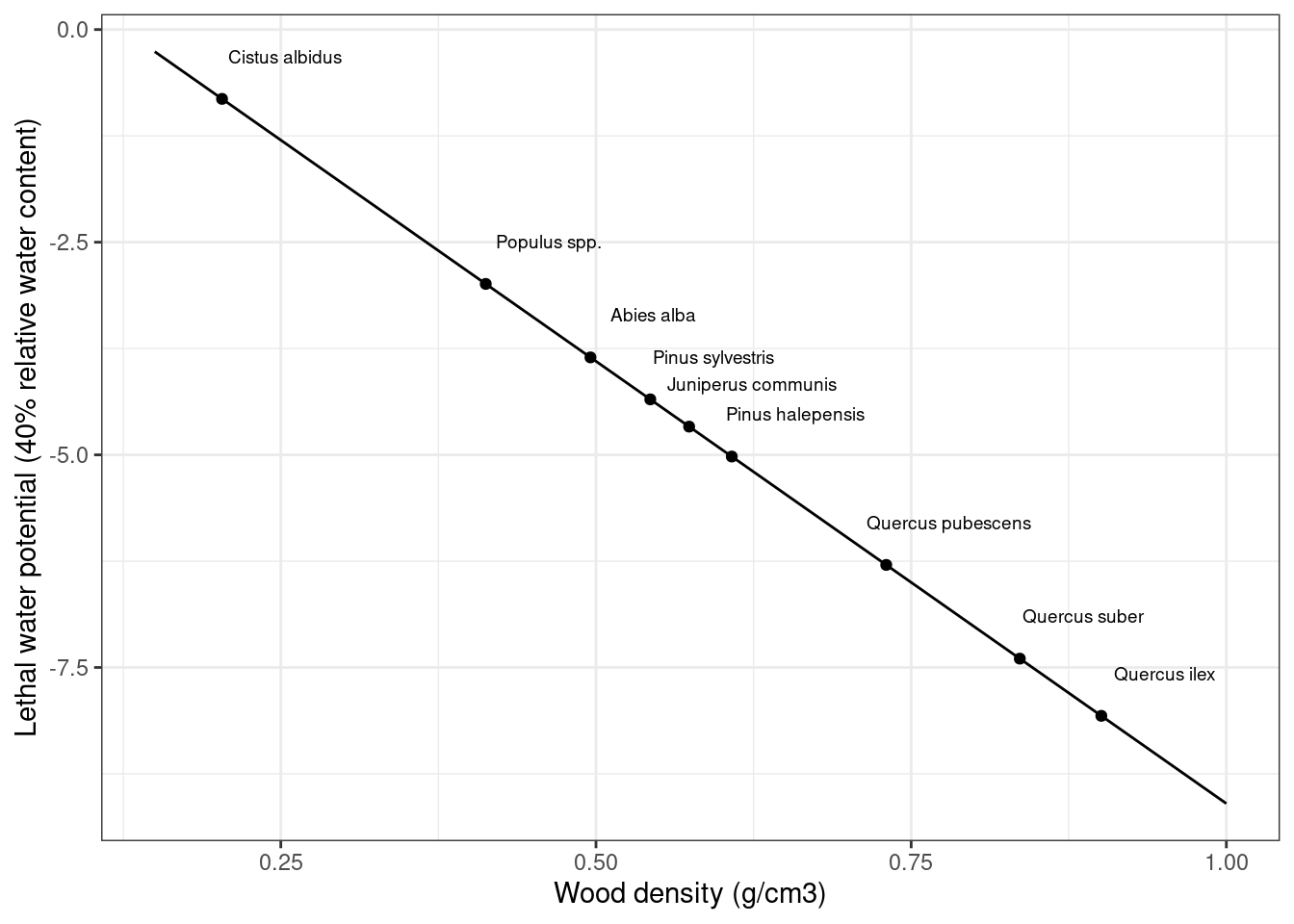
Figure 17.1: Annual (top) and daily (bottom) probability of starvation as a function of sapwood starch concentration relative to its equilibrium value.
17.5.4 Mortality due to dessication
As explained in the section 15.1.5, the dessication stress indicator (\(D_{stem}\)) is the maximum of relative water content in the stem (\(RWC_{stem}\)) and relative hydraulic conductance in the stem, i.e. the complement of \(PLC_{stem}\)
\[\begin{equation} D_{stem} = (RWC_{stem}, 1.0 - PLC_{stem})/2.0 \end{equation}\]
Assuming that a threshold of relative water content (\(RWC_{thresh}\)) corresponds to 50% annual mortality due to dessication, its probability is estimated analogously to starvation. First, a logistic sigmoidal function is used to estimate the probability of annual dessication from a given \(D_{stem}\) value:
\[\begin{equation} P_{dessic, annual} = 1.0 - \frac{\exp(40 \cdot (D_{stem} - RWC_{thresh}))}{1.0 + \exp(40 \cdot (D_{stem} - RWC_{thresh}))} \end{equation}\]
Since the model operates at the daily temporal resolution, \(P_{dessic, annual}\) is re-expressed as a daily probability using:
\[\begin{equation} P_{dessic, daily} = 1.0 - \exp(\log(1.0 - P_{dessic, annual})/356) \end{equation}\]
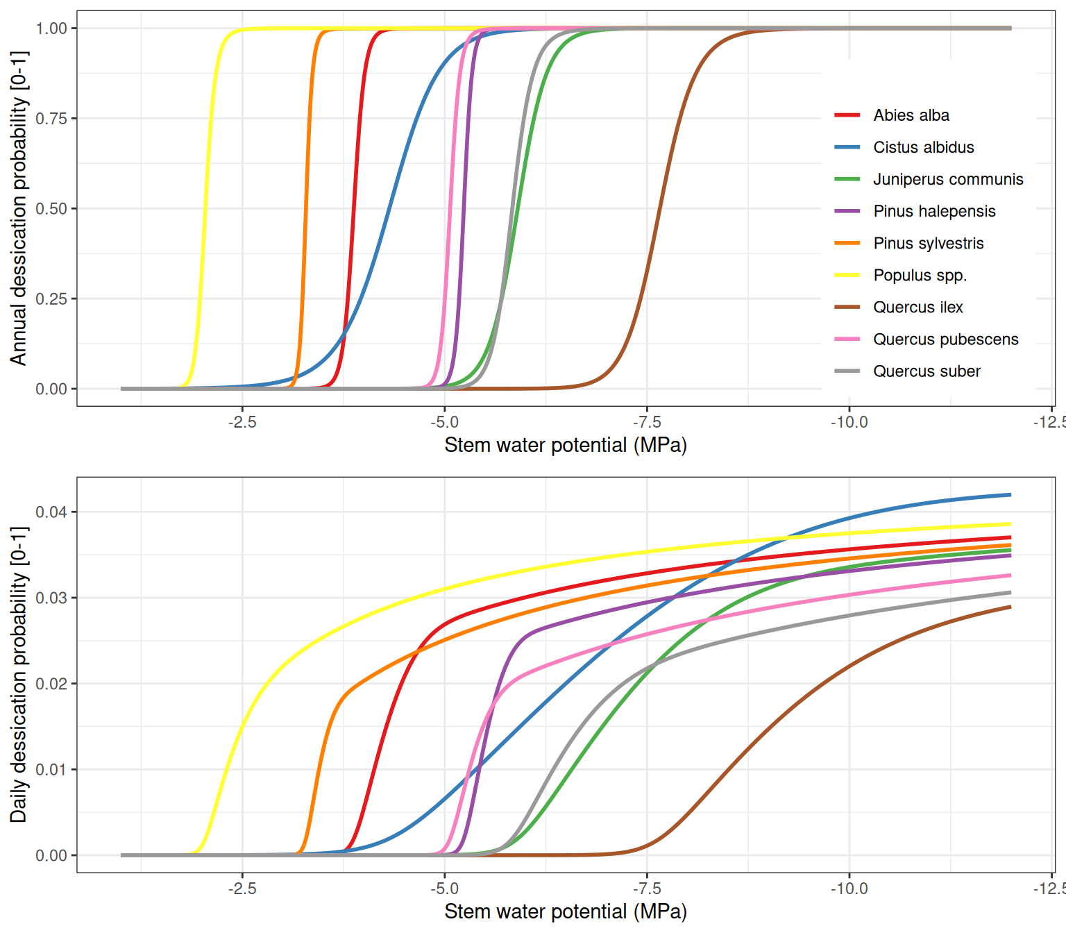
Assuming a relative threshold \(RWC_{thresh} = 0.4\), the figure below illustrates the shape of the sigmoidal function (top) and the corresponding daily probability function.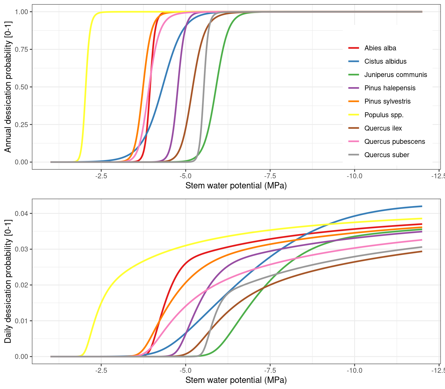
Figure 17.2: Annual (top) and daily (bottom) probability of dessication as a function of the average value of stem relative water content and stem relative hydraulic conductance.
Uncertainty of stem pressure-volume parameters
As explained in 15.1.5, using stem relative water content as indicator of dessication has the inconvenient that the parameters \(\pi_{0,stem}\) and \(\epsilon_{stem}\) specifying the pressure-volume curve are often not known, so that estimates have to come from wood density (see section A.3.14). The following figure shows the water potential corresponding to the dessication threshold for species with different wood density:

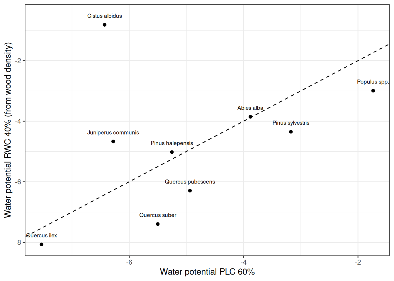
If the relationship between wood density and the stem pressure-volume curve (A.3.14) does not hold for a particular species the mortality rate may be under or overestimated. Here an example would be Cistus albidus, which has a low wood density but high dessication resistance. This is illustrated when we draw a scatter plot between the water potential corresponding to 60% stem PLC (i.e. 40% stem relative hydraulic conductance) against the water potential corresponding to 40% stem RWC:
As explained in 15.1.5, one can avoid the potential uncertainty in dessication mortality by defining the dessication stress indicator (\(D_{stem}\)) as the maximum of relative water content in the stem (\(RWC_{stem}\)) and relative hydraulic conductance in the stem. When we do so, the following curves are obtained for each of the previous species:
It is obvious in the former figure that using \(D_{stem}\) is indicator results in curves that are not continuous in all their range. However, we prefer this inconvenient to the potential overestimation of mortality due to an uncertainty in the pressure-volume curve parameters.
17.5.5 Overall mortality probability
Every day the model determines for woody cohorts the overall probability of mortality (\(P_{mort, daily}\)) as the maximum of the basal probability, starvation probability and dessication probability:
\[\begin{equation} P_{mort, daily} = \max( P_{base, daily},\, P_{starv, daily}, \, P_{dessic, daily}) \end{equation}\]
At this point \(P_{mort, daily}\) may be used deterministically (i.e., as a proportion of \(N\) to kill) or stochastically (i.e. throwing a random number between 0 and 1 to determine the mortality event).
17.6 Fire severity
Fire effects on plants follow, with some modifications, the model by Michaletz & Johnson (2008). Buoyant plume theory is first used to estimate the vertical plume temperature \(T_{plume}\) distribution that will drive heat transfer to the vascular cambium and vegetative organs. Heat transfer theory is then used to calculate the depth of vascular cambium necrosis and height of crown foliage and crown bud necrosis. Finally, these severity metrics are used to define the fate of the plant cohort, as described in section 15.1.6.
17.6.1 Plume temperature distribution
The surface fire is assumed to occur at the time of the day where temperature is \(T_{max}\) is the maximum daily temperature. For a line-source plume in a quiescent atmosphere (no wind), the plume temperature \(T_{plume}\) at height \(z\) (in m) can be estimated using (Michaletz & Johnson 2008): \[\begin{equation} T_{plume}(z) = \min{\left[900,\, C_{plume}\cdot \left( \frac{1}{z} \right) \cdot \left(\frac{T_{max} + 273.15}{g} \right)^{1/3} \cdot \left( \frac{I_{B}}{c_{p, air} \cdot \rho_{air}} \right)^{2/3} + T_{max} \right]} \tag{17.2} \end{equation}\] where \(C_{plume} = 2.6\) is the plume proportionality constant, \(g = 9.8\,m \cdot s^{-2}\) is the gravity constant, \(I_{B}\) is Byram’s surface fireline intensity (eq. (26.10); expressed in \(kW\cdot m^{-1}\)), \(c_{p, air} = 1.007\,J\cdot kg^{-1}\cdot ^{\circ} \mathrm{C}^{-1}\) is the specific heat capacity of the air and \(\rho_{air}\) is the air density at temperature \(T_{max}\). Because this similarity analysis fails at heights comparable with the fireline width, \(T_{plume}\) is constrained to a maximum flame temperature of 900 \(^{\circ} \mathrm{C}\).
17.6.2 Foliage and crown bud necrosis
The model predicting the distribution of plume temperature and the residence time of surface fires \(t_R\) (eq. (26.11)), are used to determine the height of necrosis for plant organs, here foliage or crown buds, depending also on their heat capacitance. The estimate (foliage or bud) necrosis height \(z_n\) (in m) is given by (Michaletz & Johnson 2008): \[\begin{equation} z_n = C_{plume}\cdot \left( \frac{1}{T_{crit} - T_{max}} \right) \cdot \left(\frac{T_{max} + 273.15}{g} \right)^{1/3} \cdot \left( \frac{I_{B}}{c_{p, air} \cdot \rho_{air}} \right)^{2/3} \tag{17.3} \end{equation}\] where \(T_{crit}\) is the critical temperature of the plume required for organ necrosis, given a residence time \(t_R\), which is estimated using: \[\begin{equation} T_{crit} = \frac{T_n - \theta_{T} \cdot T_{max}}{1 - \theta_{T}} \end{equation}\] Here, \(T_n\) is the temperature leading to necrosis, assumed to be \(60^{\circ}\mathrm{C}\) and \(\theta_{T}\) is defined as the excess temperature ratio, which depends on the organ thermal factor (\(TF\)) and \(t_R\): \[\begin{equation} \theta_{T} = exp(- TF \cdot t_R) \end{equation}\] The thermal factor \(TF\) is normally larger for leaves than buds, given their higher surface are to volume ratio, resulting in lower values of \(T_{crit}\) and, therefore, higher values of necrosis height. In the case of leaves, the thermal factor (\(TF_{leaves}\)) is estimated from specific leaf area, \(SLA\), using (Michaletz & Johnson 2006; Michaletz & Johnson 2008): \[\begin{equation} TF_{leaves} = SLA \cdot (h_{leaves}/c_{leaves}) \end{equation}\] where \(h_{leaves}=130\) stands for the convection heat transfer coefficient of leaves and \(c_{leaves} = 2500\) is the specific heat capacity of leaves. Typical values would be \(TF_{leaves} = 0.208\) for \(SLA = 4\) and \(TF_{leaves} = 0.624\) for \(SLA = 12\). Currently, for crown buds a constant \(TF_{buds} = 0.130\) is assumed, on the basis of values given in Michaletz & Johnson (2006), but we acknowledge that \(TF_{buds}\) should be at least species-specific. Once \(z_n\) is defined, for either leaves or crown buds, depending on their \(TF\) value, the vertical leaf distribution described in 2.4.3.3 is used to determine the proportion of crown leaves or crown buds with necrosis.
If the case of a crown fires, i.e. if surface fireline intensity is larger than van Wagner’s critical intensity; eq. (26.13), then all crown foliage is burned. The same happens if torching occurs for the target plant cohort, which is determined by calculating a cohort-specific critical intensity. Crown bud necrosis is decided in those cases by calculating \(T_{crit}\) using the crown fire residence time and comparing it to the flame temperature, i.e. \(900^{\circ}\mathrm{C}\). Despite these calculations, in practice all crown buds will also normally suffer necrosis under a crown fire.
17.6.3 Cambium necrosis
Vascular cambium necrosis is a one-dimensional transient conduction problem depending the thermal diffusivity of the bark, \(\alpha_{bark}\), and the surface fire residence time \(t_R\). Assuming that the bark surface temperature is equal to the plume temperature at \(z = 0.1\), i.e. \(T_{plume}(0.1)\), the radial bole necrosis depth, \(x_n\) (in m), can be estimated using: \[\begin{equation} x_n = 2 \cdot (\alpha_{bark} \cdot t_R)^{1/2} \cdot \mathrm{erf}^{-1}\left( \frac{T_n - T_{plume}(0.1)}{T_{max} - T_{plume}(0.1)} \right) \end{equation}\]
where \(\mathrm{erf}^{-1}\) is the inverse error function. Bark diffusivity (\(\alpha_{bark}\)) is estimated following the equations given in Michaletz & Johnson (2008), which depend on bark’s tissue density, moisture content (estimated assuming a fine dead fuel) and temperature. Cambium necrosis is determined by comparing \(x_n\) (in m) with \(x_{ba}\) (in mm) the bark thickness of the plant, which in case of trees depends on DBH: \[\begin{equation} x_{ba} = a_{bt} \cdot DBH^{b_{bt}} \end{equation}\] and in the case of shrubs \(x_{ba}\) is assumed to be equal to a fixed species-specific value \(bt_{sh}\).