Chapter 26 Fuel characteristics and fire behaviour
26.1 Overview
Functions fuel_FCCS() and fire_FCCS() allow calculating potential fire behaviour for forest inventory plots. Formulation of fuel characteristics and fire behaviour is an adaptation of the Fuel Characteristics Classification System [FCCS; Prichard et al. (2013)]. In FCCS, fuelbed is divided into six strata, including canopy, shrub, herbaceous vegetation, dead woody materials, leaf litter and ground fuels. All except ground fuels are considered here. The intensity of burning depends on several factors, including topography, wind conditions, fuel structure and its moisture content, which is determined from antecedent and current meteorological conditions. A modification of the Rothermel’s (1972) model is used to calculate the intensity of surface fire reaction (in \(kW/m^2\)) and the rate of fire spread (in \(m/min\)) of surface fires assuming a steady-state fire. Both quantities are dependent on fuel characteristics, windspeed and direction, and topographic slope and aspect.
Fuel and fire behavior calculations provide the following results:
- Fuel characteristics by stratum.
- Surface fire behavior (i.e. reaction intensity. rate of spread, fireline intensity and flame length);
- Crown fire behavior.
- Fire potential ratings of surface fire behavior and crown fire behavior.
The following figure provide an overview of the steps to calculate surface/crown fire behavior and fire potentials from fuel characteristics.
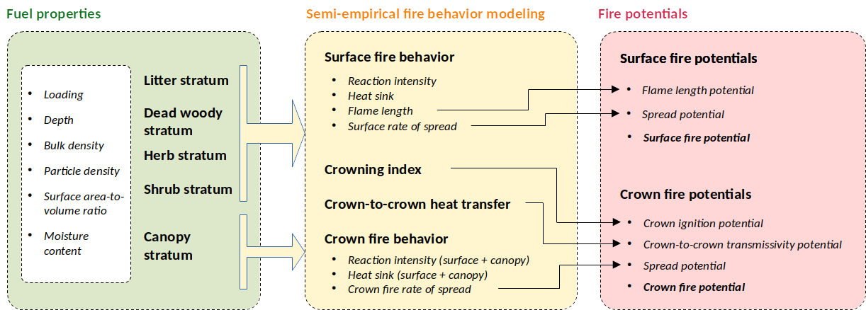
Figure 26.1: Overview of the steps involved in fire behavior and fire potential calculations starting from fuel properties
26.2 Input data
26.2.1 Forest plot data
As explained in section 2.4, medfate has been specially designed to work with forest inventory plots. The tree/shrub cohort attributes required to apply allometric models are same as for chapter 23:
| Symbol | Units | R | Description | trees | shrubs |
|---|---|---|---|---|---|
| \(SP_i\) | Species |
Species identity | Y | Y | |
| \(H_i\) | \(cm\) | Height |
Average tree or shrub height | Y | Y |
| \(N_i\) | \(ind · ha^{-1}\) | N |
Density of tree individuals | Y | N |
| \(DBH_i\) | \(cm\) | DBH |
Tree diameter at breast height | Y | N |
| \(Cover_i\) | % | Cover |
Shrub percent cover | N | Y |
Cohorts are not distinguished for the herbaceous stratum, and the variables needed are:
| Symbol | Units | R | Description |
|---|---|---|---|
| \(C_{he}\) | % | herbCover |
Herbaceous percent cover |
| \(H_{he}\) | \(cm\) | herbHeight |
Mean herb height |
Finally, the model also requires the percent cover of trees in the canopy (\(C_{ca}\)). This is easily available from forest inventory data, but could also be derived from the description of tree cohorts.
Fire behaviour functions require data in form of a forest object (see section 2.4.2).
26.2.2 Species parameters
The following functional parameters are required for each species:
| Symbol | Units | R | Description |
|---|---|---|---|
| \(L_{shape}\) | Categorical | LeafShape |
Leaf shape: “Broad”, “Needle”, “Linear”, “Scale”, “Spines” or “Succulent” |
| \(L_{size}\) | Categorical | LeafSize |
Leaf size: “Small” (< 225 mm), “Medium” (> 225 mm & < 2025 mm) or “Large” (> 2025 mm) |
| \(r_{6.35}\) | r635 |
Ratio between the weight of leaves plus branches and the weight of leaves alone for branches of 6.35 mm | |
| \(\rho_{wood}\) | \(g \cdot cm^{-3}\) | WoodDensity |
Density of wood tissue |
| \(\rho_{leaf}\) | \(g \cdot cm^{-3}\) | LeafDensity |
Density of leaf tissue |
| \(\sigma_{i}\) | \(m^2 \cdot m^{-3}\) | SAV |
Surface-area-to-volume ratio of the small fuel (1h) fraction (leaves and branches < 6.35mm) |
| \(h\) | \(kJ \cdot kg^{-1}\) | HeatContent |
High fuel heat content. |
| \(LD\) | years | LeafDuration |
Leaf duration (in years) |
| \(LI\) | % | PercentLignin |
Percentage of lignin in leaves |
Leaf shape and size categories are used to determine leaf litter fuel types.
26.2.3 Other inputs
Other inputs may be given by expert opinion or they may be calculated from another model. Specifically, for each plant cohort (and for any day of application) the fire behaviour model requires:
- \(P_{dead}\): Proportion of the plant that is dead.
- \(FMC\): Fuel moisture content (in percent of dry weight).
Analogously, the same variables are needed for the herbaceous stratum.
- \(P_{dead,he}\): Proportion of herb fuels that respond to humidity changes as 1-h dead fuels.
- \(FMC_{live,he}\): Fuel moisture content of live herb fuels (in percent of dry weight).
The model also needs the following input parameters:
- \(FMC_{dead}\): the moisture content of 1-h dead fuels (in percent of dry weight).
- \(U\): Midflame windspeed (in \(m\cdot s^{-1}\)).
- \(S\): Slope (in percent).
26.3 Fuel characteristics
26.3.1 Fuel strata
The Fuel Characteristics Classification System (FCCS) on which this document is based, defines six fuel strata (Prichard et al. 2013):
- Canopy: Trees, snags and ladder fuels.
- Shrubs: Primary and secondary layers.
- Non-woody vegetation (herbs): grasses, sedges, rushes and forbs.
- Woody fuels: All downed and dead wood, sound wood, rotten wood and stumps.
- Litter-lichen-moss: Lichen, litter and moss layers.
- Ground fuels: Duff, basal accumulation and squirrel middens.
Shrubs, herbs and woody fuels are constitute the upper surface fuels, whereas herbs and woody fuels alone consitute the lower surface fuels. FCCS summarizes and calculates characteristics for each fuelbed stratum and layer. Our model estimates fuel loading and characteristics for canopy, shrub, non-woody vegetation, as well as fine (1h) woody fuels and litter fuels. Larger woody fuels (10h or 100h) could be considered if information about forest management actions is available. Ground fuels are not included here.
26.3.2 Cohort fuel loading
Here we consider as burnable fuels foliage and branches up to 6.35 mm = 0.25 in in diameter. The same consideration applies to both trees and shrubs. They are calculated from forest objects using function plant_fuel().
Tree cohorts
Fine fuel loading for a tree cohort (\(W_{i}\); in \(kg\cdot m^{-2}\)), including its leaves and branches with diameter up to 6.35 mm = 0.25 in, is calculated from foliar biomass (\(FB_{i}\), see eq. (23.2)) using: \[\begin{equation} W_{i} = r_{6.35,i}\cdot FB_{i} \end{equation}\] where \(r_{6.35,i}\) is the ratio between the weight of leaves plus branches and the weight of leaves alone for branches of 6.35 mm in diameter for the species of cohort \(i\). The biomass corresponding to branches of less than < 6.35 mm (\(SBB_{i}\), also in \(kg\cdot m^{-2}\)) is obtained by subtraction: \[\begin{equation} SBB_{i} = (r_{6.35,i}-1)\cdot FB_{i} \end{equation}\] Whereas \(W_{i}\) is the cohort loading variable influencing fire behavior, \(FB_{i}\) and \(SBB_{i}\) are cohort variables used to estimate fine dead woody and leaf litter loadings.
Shrub cohorts
Our procedure to estimate shrub fuel loading differs from Prichard et al. (2013) because they calculate first total biomass of the shrub species and then consider the percentage of total weight that corresponds to leaves and small branches. In our case, we estimate fine fuel loading (\(W_{i}\), in \(kg \cdot m^{-2}\)) and foliar biomass (\(FB_i\), in \(kg \cdot m^{-2}\)) of shrubs from eqs. (23.4) and (23.5). Biomass of small branches (in \(kg \cdot m^{-2}\)) can be obtained from : \[\begin{equation} SBB_{i} = W_{i} - FB_{i} \end{equation}\]
26.3.3 Vertical distribution of cohort fuels
Vertical distribution of fine fuels are distributed between the crown base height (\(H_{crown,i}\); in \(cm\)) and the total height (\(H_i\), in \(cm\)) following a truncated Gaussian distribution, as done for the distribution of leaves (see section 2.4.3.3). Crown base height of trees is calculated as explained in 23.2.3. The loading of a cohort that occurs within a given height interval of limits \(H_1\) and \(H_2\) is calculated as: \[\begin{equation} W_i(H_1, H_2) = W_i\cdot p_i(H_1, H_2) \end{equation}\] where \(p_i(H_1, H_2)\) is the proportion of the crown of cohort \(i\) that corresponds to the height interval \((H_1, H_2)\).
26.3.4 Fuel bulk density profile
Knowing at which height fuels are placed, the fuel bulk density profile (Reinhardt et al. 2006) is defined for any given interval \((H_1, H_2)\) as the bulk density (\(kg/m^3\)) of fine fuels corresponding to that interval: \[\begin{equation} BDP(H_1, H_2) = \frac{\sum_{i} W_i(H_1, H_2)}{H_2-H_1} \end{equation}\] Canopy bulk density normally ranges between 0 and 0.4 \(kg/m^3\) (Scott & Reinhardt 2002). Sando & Wick (1972) arbitrarily defined canopy base height as the lower vertical 0.3-m section with a weight greater than \(0.01124 kg/m^3\). A user-defined threshold \(t_{BDP}\) (in \(kg/m^3\)) in 0.1-m sections is used to differentiate the surface fuelbed from canopy fuels. Using this threshold the model calculates the following three heights (Reinhardt et al. 2006):
- Shrub stratum base height, \(H_{sb}\) (in \(cm\)): the minimum height between 0 and 2 m where fuel bulk density is larger than \(t_{BDP}\).
- Shrub stratum top height, \(H_{st}\) (in \(cm\)): the maximum height between 0 and 2 m where fuel bulk density larger than \(t_{BDP}\). With this definition \(h_{s}\) cannot be higher than 2 m (corresponding to fuel model 4 in Anderson 1982).
- Canopy base height, \(H_{cb}\) (in \(cm\)): In terms of its consequences to crown fire initiation, canopy base height can be defined as the lowest height above the ground at which there is sufficient canopy fuel to propagate fire vertically through the canopy. It is calculated as the minimum height over \(H_st\) when the bulk density starts again to be larger than \(t_{BDP}\).
- Canopy top height, \(H_{ct}\) (in \(cm\)): the maximum height where bulk density is larger than \(t_{BDP}\).
- Canopy gap, \(H_{gap}\) (in \(cm\)): the difference between \(H_{cb}\) and \(H_{st}\). The canopy gap is used to calculate crown initiation potential.
vprofile_fuelBulkDensity()). Following Mitsopoulos & Dimitrakopoulos (2007), a threshold \(t_{BDP} = 0.04\) is used to determine shrub and canopy heights.
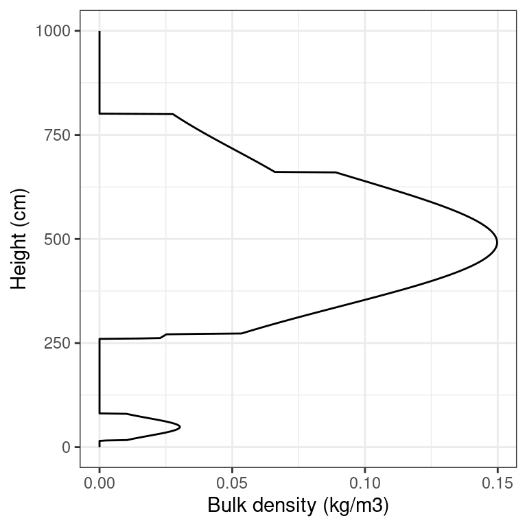
Figure 26.2: Bulk density profile of an example forest
26.3.5 Fuel loading (\(w\)) and fuel depth (\(\delta\))
26.3.5.1 Canopy stratum
Canopy loading (in \(kg\cdot m^{-2}\)) is the sum of (tree and shrub) cohort loadings above 2 m (i.e. 200 cm): \[\begin{equation} w_{ca} = \sum_{i}w_{i,ca} =\sum_{i}{W_i(200, \infty}) \end{equation}\] where \(w_{i,ca}\) is the canopy stratum loading of cohort \(i\). Canopy depth (in \(m\)) is defined as the average of tree (or shrub) crown lengths above 2 m, weighted by the loadings of cohorts in the canopy: \[\begin{equation} \delta_{ca} = \frac{1}{100}\cdot\frac{\sum_{i}{w_{i,ca}\cdot (H_i - H_{b,i})\cdot p_{i,ca} }}{\sum_{i}{w_{i,ca}}} \end{equation}\] where the proportion of a tree (or shrub) cohort in the canopy stratum is \(p_{i,ca}=p_{i}(200,\infty)\).
26.3.5.2 Shrub stratum
Shrub loading (in \(kg\cdot m^{-2}\)) is the sum of (tree and shrub) cohort loadings between the ground and 2 m (i.e. 200 cm): \[\begin{equation} w_{sh} = \sum_{i}w_{i,sh} =\sum_{i}W_i(0, 200) \end{equation}\] where \(w_{i,sh}\) is the shrub stratum loading of cohort \(i\). The depth of the shrub stratum (in \(m\)) is defined as the average of tree (or shrub) crown lengths below 2 m, weighted by the loadings of cohorts in the shrub stratum: \[\begin{equation} \delta_{sh} = \frac{1}{100}\cdot \frac{\sum_{i}{w_{i,sh}\cdot (H_i - H_{b,i})\cdot p_{i,sh} }}{\sum_{i}{w_{i,sh}}} \end{equation}\] where the proportion of a shrub (or tree) cohort in the shrub stratum is \(p_{i,sh}=p_{i}(0,200)\).
26.3.5.3 Non-woody stratum
Herb percent cover and average herb height are transformed into herbaceous loading (\(kg\cdot m^{-2}\)) using (ref piropinos): \[\begin{equation} w_{he} = 0.014 \cdot C_{he} \cdot (H_{he}/100) \end{equation}\] The depth of the herbaceous stratum (in \(m\)) is simply the mean height of herbs: \[\begin{equation} \delta_{he} = H_{he}/100 \end{equation}\]
26.3.5.4 Woody and litter strata
In FCCS (Prichard et al. 2013), woody surface loading includes several fuel sizes. However, when calculating surface fire behavior \(w_{wo}\) includes 100% of 1h fuels, 25% of 10h fuels and 12.5% of 100h fuels, which represents the material available for flaming combustion. Obtaining loading estimates for 10h- and 100h-fuels is very difficult without field fuel sampling. However, we might estimate 1h woody fuels and leaf litter from standing biomass of small branches (< 6.35mm) and leaves for trees and shrubs. Hence, our treatment of surface woody fuels includes only fine (1h) fuels.
Assuming a continuous input of litter, the variation in accumulated litter is described by a simple differential equation (Birk & Simpson 1980): \[\begin{equation} \frac{\mathrm{d}X}{\mathrm{d}t} = L - k\cdot X \end{equation}\] where \(k\) is the decay constant, \(L\) is the rate of litterfall and \(X\) is the litter mass accumulated in the forest floor. Assuming that litter mass has reached a steady state, \(X\) can be estimated as the ratio between \(L\) and \(k\). If litterfall is estimated as the total foliar biomass divided by leaf duration, the amount of steady state leaf litter corresponding to each tree and srhub cohort can be estimated using: \[\begin{equation} w_{li, i} = \frac{FB_i}{LD(SP_i) \cdot k_i} \end{equation}\] where \(FB_i\) is the foliar biomass of cohort \(i\), \(LD(SP_i)\) is the species-specific average leaf duration (in years) and \(k_i\) is the rate of decay of leaves of cohort \(i\), which is given by the regreession model of Meentemeyer (1978): \[\begin{equation} k_i = (-0.5365+0.00241\cdot AET) - (-0.01586+0.000056\cdot AET) \cdot LI(SP_i) \end{equation}\] where \(LI(SP_i)\) is the species-specific percentage of lignin content in leaves and AET is actual evapotranspiration (default \(AET = 1000 mm\)). Litter loadings are summed for four litter types (short pine needles, long pine needles, other conifers, broadleaves). In the case of fine dead woody materials (small fallen branches), loading of small branches is taken as woody litter and it is assumed that small branch litterfall occurs at the same time as leaf litterfall (i.e. according to leaf duration): \[\begin{equation} w_{wo} = \sum_{i}{w_{wo, i}} = \sum_{i}{\frac{SBB_i}{LD(SP_i)\cdot k_{wo}} } \end{equation}\] where \(k_{wo} = 0.95 y^{-1}\) is a constant rate of decomposition for small branches.
In FCCS, the depth of woody and LLM strata are inputs. In our case the depth of the woody and litter strata are estimated from the corresponding fuel loadings: \[\begin{eqnarray} \delta_{wo} &=& w_{wo}/\rho_{b, wo}\\ \delta_{li} &=& w_{li}/\rho_{b, li} \end{eqnarray}\] where \(\rho_{b, wo}\), \(\rho_{b, li}\) are the woody and litter bulk density (in \(kg\cdot m^{-3}\)), respectively. Litter bulk density \(\rho_{b,li}\) is calculated as a weighted average of litter types: \[\begin{equation} \rho_{b,li} = \frac{\sum_{k}{ \rho_{b,k}\cdot w_{li,k}}}{\sum_{k} {\cdot w_{li,k}}} \end{equation}\] where \(k\) indicates litter type. The bulk density for litter types are [Prichard et al. (2013); Table 1]: \[\begin{eqnarray} \rho_{b,shortneedlepine} &=& \rho_{b,longneedlepine} = \rho_{b,otherconifer}= 1.65 lb\cdot ft^{-3} = 26.43 kg\cdot m^{-3}\\ \rho_{b,hardwood} &=& 0.83 lb\cdot ft^{-3} = 13.30 kg\cdot m^{-3} \end{eqnarray}\]
26.3.6 Other fuel characteristics
All the following characteristics are calculated in metric units (although British units are indicated to qualify specific values for compatibility).
26.3.6.1 Particle density (\(\rho_{p}\))
Particle density is the ratio of dry weight over volume for fuel particles (in \(kg\cdot m^{-3}\)). When species have different values, particle density averages for shrub and canopy strata can be obtained as: \[\begin{eqnarray} \rho_{p, sh} &= \frac{\sum_{i}{w_{i,sh} \cdot \rho_p(SP_i)}}{\sum_{i}{w_{i,sh}}}\\ \rho_{p, ca} &= \frac{\sum_{i}{w_{i,ca} \cdot \rho_p(SP_i)}}{\sum_{i}{w_{i,ca}}} \end{eqnarray}\] where \(\rho_p(SP_i)\) is the species-specific particle density (in \(kg\cdot m^{-3}\)), which can be obtained from wood tissue (\(\rho_{wood}\)) and leaf tissue (\(\rho_{leaf}\)) densities, using \(r_{6.35}\) to weight them: \[\begin{equation} \rho_p(SP_i) = 1000 \cdot (\rho_{leaf}(SP_i)\cdot f_{leaves,vol} + \rho_{wood}(SP_i)\cdot (1 - f_{leaves,vol})) \end{equation}\] where \(f_{leaves,vol}\) is the volumetric fraction of leaves with respect to branchlets: \[\begin{equation} f_{leaves,vol} = \left[1.0 +(r_{6.35}(SP_i) - 1.0) \cdot \frac{\rho_{wood}(SP_i)}{\rho_{leaf}(SP_i)} \right]^{-1} \end{equation}\]
Dead woody and litter particle densities, i.e. \(\rho_{p, wo}\) and \(\rho_{p, li}\), are obtained averaging wood tissue and leaf tissue densities across cohorts: \[\begin{eqnarray} \rho_{p, wo} &= \frac{\sum_{i}{w_{i} \cdot \rho_{wood}(SP_i)}}{\sum_{i}{w_{i}}}\\ \rho_{p, li} &= \frac{\sum_{i}{w_{i} \cdot \rho_{leaf}(SP_i)}}{\sum_{i}{w_{i}}}\\ \end{eqnarray}\] Finally, herb particle density, \(\rho_{p, he}\), is set to a default value \(\rho_{p,he} = 400 kg\cdot m^{-3}= 25 lb\cdot ft^{-3}\) (Prichard et al. 2013).
26.3.6.2 Particle volume (\(PV\))
Particle volume is defined as the volume of particles per surface area (in \(m^3\cdot m^{-2}\)). Is calculated as dry weight loading divided by particle density. If species have different particle density values, the particle volume for canopy (\(PV_{ca}\)) and shrub(\(PV_{sh}\)) strata can be calculated using: \[\begin{eqnarray} PV_{ca} &= \sum_{i}{PV_{i,ca}} = \sum_{i}{w_{i,ca}/\rho_{p}(SP_i)}\\ PV_{sh} &= \sum_{i}{PV_{i,sh}} = \sum_{i}{w_{i,sh}/\rho_{p}(SP_i)} \end{eqnarray}\] where \(PV_{i,ca}\) and \(PV_{i,sh}\) are the particle volume of cohort \(i\) in the canopy and shrub strata, respectively. The particle volume for woody and herb strata are simply: \[\begin{eqnarray} PV_{wo} &= w_{wo}/\rho_{p,wo}\\ PV_{he} &= w_{he}/\rho_{p,he} \end{eqnarray}\] The particle volume for the litter stratum is the sum of particle volume of litter components: \[\begin{equation} PV_{li} = \sum_{i}{PV_{li,k}} = \sum_{i}{w_{li,k}/\rho_{p, li}} \end{equation}\]
26.3.6.3 Packing ratio (\(\beta\))
The proportion of fuelbed stratum volume occupied by fuel particles is an important factor to predict fire behavior. At low packing ratios (low particle density) fire intensity is limited by excessive heat loss. At high packing ratios (high particle density), lack of oxygen limits combustion. The packing ratios for the canopy and shrub stratum (\(\beta_{ca}\) and \(\beta_{sh}\); dimensionless) are given by: \[\begin{eqnarray} \beta_{ca} &=& \frac{PV_{ca}}{\delta_{ca}}\\ \beta_{sh} &=& \frac{PV_{sh}}{\delta_{sh}} \tag{26.1} \end{eqnarray}\] where \(w_{i,ca}\) and \(w_{i,sh}\) are the contribution of cohort \(i\) to canopy and shrub strata loading (in \(kg\cdot m^{-2}\)), respectively, and \(\rho_p(SP_i)\) is the particle density (in \(kg\cdot m^{-3}\)) of fuels in cohort \(i\). The packing ratio for the herbaceous, woody and litter strata are: \[\begin{eqnarray} \beta_{he} &=& \frac{PV_{he}}{\delta_{he}}\\ \beta_{wo} &=& \frac{PV_{wo}}{\delta_{wo}} = \frac{\rho_{b,wo}}{\rho_{p,wo}}\\ \beta_{li} &=& \frac{PV_{li}}{\delta_{li}} = \frac{\rho_{b,li}}{\rho_{p,li}} \end{eqnarray}\] Note that the packing ratio expressions for woody and litter strata as a ratio of bulk and particle density arises as a consequence of how fuel depth and particle volume are estimated.
26.3.6.4 Surface-area-to-volume ratio (\(\sigma\))
The surface-area-to-volume ratio (in \(m^2\cdot m^{-3}\)) for the canopy or shrub strata are calculated using weighted averages: \[\begin{eqnarray} \sigma_{ca} &=& \frac{\sum_{i}{w_{i,ca} \cdot \sigma(SP_i)}}{\sum_{i}{w_{i,ca}}}\\ \sigma_{sh} &=& \frac{\sum_{i}{w_{i,sh} \cdot \sigma(SP_i)}}{\sum_{i}{w_{i,sh}}} \end{eqnarray}\] where \(w_{i,ca}\) and \(w_{i,sh}\) are the contribution of cohort \(i\) to canopy and shrub strata loading (in \(kg\cdot m^{-2}\)), respectively, and \(\sigma(SP_i)\) is the species-specific surface-area-to-volume ratio. The surface-area-to-volume ratio of herbs is assumed constant \(\sigma_{he} = 11483 m^2\cdot m^{-3} = 3500 ft^2\cdot ft^{-3}\) and that of small (1-h) woody fuels is \(\sigma_{wo} = 1601.05 m^2\cdot m^{-3} = 488 ft^2\cdot ft^{-3}\). The surface-area-to-volume ratio for the litter stratum is: \[\begin{equation} \sigma_{li} = \frac{\sum_{k}{w_{li,k} \cdot \sigma_{k}}}{\sum_{k}{w_{li,k}}} \end{equation}\] and the surface-area-to-volume ratio for litter types are: \[\begin{eqnarray} \sigma_{shortneedlepine} &= 6562 m^{2}\cdot m^{-3}= 2000 ft^{2}\cdot ft^{-3}\\ \sigma_{longneedlepine} &= 4921 m^{2}\cdot m^{-3}= 1500 ft^{2}\cdot ft^{-3}\\ \sigma_{otherconifer} &= 8202 m^{2}\cdot m^{-3}= 2500 ft^{2}\cdot ft^{-3}\\ \sigma_{hardwood} &= 8202 m^{2}\cdot m^{-3}= 2500 ft^{2}\cdot ft^{-3} \end{eqnarray}\]
26.3.6.5 Fuel area index (FAI)
The fuel area index (FAI) is the total fuel surface area per unit of ground area (unitless). It is analogous to leave area index (LAI), and it is used to calculate FCCS fire potentials (Schaaf et al. 2007). For shrub and canopy strata, FAI is calculated as: \[\begin{eqnarray} FAI_{ca} &=& \sum_{i}{FAI_{i, ca}} = \sum_{i}{PV_{i,ca} \cdot\sigma(SP_i)}\\ FAI_{sh} &=& \sum_{i}{FAI_{i, sh}}= \sum_{i}{PV_{i,sh} \cdot \sigma(SP_i)} \end{eqnarray}\] where \(FAI_{i, ca}\) and \(FAI_{i, sh}\) are the FAI of cohort \(i\) in the canopy and shrub strata, respectively. The FAI of herbs and woody strata are given by: \[\begin{eqnarray} FAI_{he} &=& PV_{he} \cdot \sigma_{he}\\ FAI_{wo} &=& PV_{wo} \cdot \sigma_{wo} \end{eqnarray}\] For the litter layer, FAI is calculated as a sum of FAI for litter components: \[\begin{equation} FAI_{li} = \sum_{k}{FAI_{li,k}} = \sum_{k}{PV_{li,k} \cdot \sigma_{k}} \end{equation}\]
26.3.6.6 Moisture content (\(FMC\))
Fuel moisture content (\(FMC\) in percent of dry weight) is averaged across cohorts composing the shrub or canopy strata, to obtain \(FMC_{live, sh}\) and \(FMC_{live, ca}\) : \[\begin{eqnarray} FMC_{live, sh} &=& \frac{\sum_{i}{w_{i,sh} \cdot FMC_i}}{\sum_{i}{w_{i,sh}}} \\ FMC_{live, ca} &=& \frac{\sum_{i}{w_{i,ca} \cdot FMC_i}}{\sum_{i}{w_{i,ca}}} \end{eqnarray}\] Live fuel moisture of herb stratum (\(FMC_{live, he}\)) is an input. The moisture of dead plant in the canopy and shrub layers (\(FMC_{dead, ca}\) and \(FMC_{dead, sh}\)), the moisture of dead herbs (\(FMC_{dead, he}\)), as well as that of litter (\(FMC_{li}\)) and woody (\(FMC_{wo}\)) strata are all assumed equal to the moisture of 1-h dead fuels, which is an input of the model.
26.3.6.7 Proportion of dead fuel (\(P_{dead}\))
Woody and litter strata are dead fuels, but for canopy, shrub and herb strata the proportion of fuels that are dead are variable. The proportion of dead fuels in the herbaceous stratum (\(P_{dead,he}\)) is an input of the model, but for the shrub and canopy strata these are calculated from the proportion of dead fuels in each cohort: \[\begin{eqnarray} P_{dead,sh} &=& \frac{\sum_{i}{w_{i,sh} \cdot P_{dead,i}}}{\sum_{i}{w_{i,sh}}} \\ P_{dead, ca} &=& \frac{\sum_{i}{w_{i,ca} \cdot P_{dead,i}}}{\sum_{i}{w_{i,ca}}} \end{eqnarray}\]
26.3.6.8 Low heat content (\(h\))
The low fuel heat content of each surface fuel stratum (in \(kJ\cdot kg^{-1}\)) is used for the calculation of reaction intensity. Heat content values are adjusted for live foliar moisture content in canopy, shrub and herb strata; and are left to the default value for woody and litter strata: \[\begin{eqnarray} h_{ca} &=& h_{ca, def} - (M_{live, ca}/100)\cdot V \\ h_{sh} &=& h_{sh, def} - (M_{live, sh}/100)\cdot V \\ h_{he} &=& h_{def} - (M_{live, he}/100)\cdot V \\ h_{wo} &=& h_{li} = h_{def} \end{eqnarray}\] where \(h_{def} = 18608 kJ\cdot kg^{-1} = 8000 Btu\cdot lb^{-1}\) is the default low heat content value for herbs, woody and litter strata, and \(V = 2596 kJ\cdot kg^{-1} = 1116 Btu\cdot lb\) is the latent heat of vaporisation of water. The default low heat of contents for the canopy and shrub strata (\(h_{ca, def}\) and \(h_{sh, def}\)) are calculated as a weighted average across cohorts: \[\begin{eqnarray} h_{ca, def} &=& \frac{\sum_{i}{w_{i,ca} \cdot h(SP_i)}}{\sum_{i}{w_{i,ca}}}\\ h_{sh, def} &=& \frac{\sum_{i}{w_{i,sh} \cdot h(SP_i)}}{\sum_{i}{w_{i,sh}}} \end{eqnarray}\] where \(h(SP_i)\) is a species-specific low heat content value.
26.3.6.9 Reactive volume (\(RV\))
The volume per surface unit (\(m^3\cdot m^{-2}\)) that would be involved in flaming combustion. \[\begin{eqnarray} RV_{sh} &=& w_{shrub}/\rho_{p, sh}\\ RV_{he} &=& w_{he}/\rho_{p, he}\\ RV_{wo} &=& w_{wo}/\rho_{p, wo}\\ RV_{li} &=& \min(w_{li}, w_{\max,li})/\rho_{p, li} \end{eqnarray}\] In the case of litter, the flame loading is limited by \(w_{\max,li}\), the maximum loading that would be consumed in the flaming stage of combustion, calculated as a weighted average of litter types: \[\begin{equation} w_{\max,li} = \frac{\sum_{k}{ w_{\max,k}\cdot w_{li,k}}}{\sum_{k} {\cdot w_{li,k}}} \end{equation}\] where \(k\) indicates litter type. The maximum combustion loadings for litter types are [Prichard et al. (2013); Table 2]: \[\begin{eqnarray} w_{\max,shortneedlepine} &=& w_{\max,otherconifer} = 0.3248 kg \cdot m^{-2} = 2900 lb\cdot ac^{-1} \\ w_{\max,longneedlepine} &=& 0.6496 kg \cdot m^{-2}= 5800 lb\cdot ac^{-1} \\ w_{\max,hardwood} &=& 0.3472 kg \cdot m^{-2}= 3100 lb\cdot ac^{-1} \end{eqnarray}\]
26.3.7 Unit conversion of fuel characteristics
FCCS calculations employ empirical equations that were derived in British units system. Hence, all the fuel characteristics and model inputs that are in metric units have to be translated into British units prior to fire behaviour calculations:
- Loading: \(1 kg\cdot m^{-2} = 0.204918 lb\cdot ft^{-2}\)
- Depths: \(1m = 3.2808399ft\)
- Particle density and bulk density: \(1 kg\cdot m^{-3} = 0.06242796 lb\cdot ft^{-3}\)
- Particle volume and reactive volume: \(1 m^{3}\cdot m^{-2} = 3.2808399 ft^{3}\cdot ft^{-2}\)
- Surface-to-area-volume ratio: \(1 m^{2}\cdot m^{-3} = 0.3048 ft^{2}\cdot ft^{-3}\)
- Heat content: \(1kJ\cdot kg^{-1} = 0.429922614 Btu\cdot lb^{-1}\)
- Wind speed: \(1 m \cdot s^{-1} = 2.23693629 mph\)
26.4 Surface fire behavior
26.4.1 Surface rate of spread (\(R\))
In the Rothermel (1972) model, surface rate of spread is defined as the ratio of heat source (i.e. the surface fire energy propagated to unburned fuels) to surface fuel heat sink (i.e. the energy required to preheat fuels). Owing to the difference in packing ratio between the litter stratum and the other surface fuels, litter-dominated fuelbeds may have substantially different spread rates than other fuelbeds. For this reason, in FCCS the rate of spread (in \(ft \cdot min^{-1}\)) is calculated separately for litter stratum and the final rate of spread is the maximum of the rate of spread of all surface fuels and that of the litter stratum. Rate of spread is also limited to a maximum based in windspeed and slope. \[\begin{equation} R = \min(WindSlopeCap, \max(R_{surf}, R_{litter})) \end{equation}\] The surface fuel and litter fuel rates of spread are given by the application of Rothermel’s (1972) equation to each case: \[\begin{eqnarray} R_{surf} &=& \frac{I_{R,surf} \cdot \xi_{surf}\cdot (1 + \phi_W + \phi_S)}{q_{surf}}\\ R_{litter} &=& \frac{I_{R,litter} \cdot \xi_{litter}\cdot (1 + \phi_W + \phi_S)}{q_{litter}} \end{eqnarray}\] where \(I_{R,surf}\) and \(I_{R,litter}\) are the reaction intensities (in \(Btu \cdot ft^{-2} \cdot min^{-1}\)), \(\xi_{surf}\) and \(\xi_{litter}\) are the propagating flux ratios, \(q_{surf}\) and \(q_{litter}\) are the heat sinks. Finally, \(\phi_W\) and \(\phi_S\) are the slope and wind modifiers. All of them are explained in the following sections. The maximum rate of spread calculated from windspeed and slope is: \[\begin{equation} WindSlopeCap = 88 \cdot U \cdot (1 + \phi_S) \end{equation}\] where \(U\) is windspeed (in \(mph\)) and \(88\) is a conversion factor (from \(mph\) to \(ft/min\)).
26.4.1.1 Reaction intensity (\(I_R\))
Reaction intensity of surface fuels (in \(Btu \cdot ft^{-2} \cdot min^{-1}\)) is calculated as the sum of component reaction intensities of the four different surface fuel strata, whereas the reaction intensity in the litter uses this strata alone: \[\begin{eqnarray} I_{R,surf} &=& I_{R, sh} + I_{R, he}+ I_{R, wo}+I_{R, li}\\ I_{R,litter} &=& I_{R, li} \tag{26.2} \end{eqnarray}\]
Each component reaction intensity is calculated using: \[\begin{eqnarray} I_{R,sh} &=& (\eta_{\beta_{allsurf}'})^{A_{sh}}\cdot \Gamma_{\max, sh}'\cdot w_{sh} \cdot h_{sh} \cdot \eta_{FMC,sh}\cdot \eta_{K,sh}\\ I_{R,he} &=& (\eta_{\beta_{lowsurf}'})^{A_{he}}\cdot \Gamma_{\max, he}'\cdot w_{he} \cdot h_{he} \cdot \eta_{FMC,he}\cdot \eta_{K,he}\\ I_{R,wo} &=& (\eta_{\beta_{lowsurf}'})^{A_{wo}}\cdot \Gamma_{\max, wo}'\cdot w_{wo} \cdot h_{wo} \cdot \eta_{FMC,wo}\cdot \eta_{K,wo}\\ I_{R,li} &=& (\eta_{\beta_{litter}'})^{A_{li}}\cdot \Gamma_{\max, li}'\cdot w_{li} \cdot h_{li} \cdot \eta_{FMC,li}\cdot \eta_{K,li} \tag{26.3} \end{eqnarray}\]
In the above equations, \(w_{sh}\), \(w_{he}\), \(w_{wo}\) and \(w_{li}\) are the loadings of the corresponding shrub, herb, woody and litter strata, respectively. These quantities were defined in previous sections, as were the corresponding low heat fuel contents (\(h_{sh}\), \(h_{he}\), \(h_{wo}\) and \(h_{li}\)). Mineral damping coefficient (\(\eta_{K}\); dimensionless) is set to the same value (corresponding to the conventional value for silica-free ash content of 1%) for all strata: \[\begin{equation} \eta_{K,sh} = \eta_{K,he} =\eta_{K,wo} = \eta_{K,li} = 0.42 \end{equation}\] In the following subsections, we describe the calculation of the remaining variables for each stratum: reaction efficiency (\(\eta_{\beta'}\)), Rothermel’s \(A\) parameter, maximum reaction velocity (\(\Gamma_{\max}'\)) and moisture damping coefficient (\(\eta_{FMC}\)).
26.4.1.2 Reaction efficiency (\(\eta_{\beta'}\))
Reaction efficiency (between 0 and 1) represents the damping effect of inefficiently packed fuels in the reaction intensity. Because shrubs rarely burn without lower surface fuels, the reaction efficiency of the surface layer (\(\eta_{\beta_{allsurf}'}\)) includes shrubs, herbs and woody fuels. Low surface fuels may carry flames without involving shrubs, so are assumed to burn with a single reaction efficiency (\(\eta_{\beta_{lowsurf}'}\)) determined by the combined characteristics of herb and woody fuel strata. Both are calculated similarly: \[\begin{eqnarray} \eta_{\beta_{allsurf}'} &=& \beta_{allsurf}'\cdot e^{1- \beta_{allsurf}'}\\ \eta_{\beta_{lowsurf}'} &=& \beta_{lowsurf}'\cdot e^{1- \beta_{lowsurf}'} \tag{26.4} \end{eqnarray}\] where \(\beta_{allsurf}'\) and \(\beta_{lowsurf}'\) are the relative packing ratios corresponding to all surface fuels and low surface fuels, respectively. Relative packing ratios (\(\beta'\); dimensionless) are defined as the ratio of optimum depth (\(\delta_{opt}\)) to effective depth (\(\delta_{eff}\)): \[\begin{eqnarray} \beta_{allsurf}' &=& \delta_{opt, allsurf} / \delta_{eff, allsurf} \\ \beta_{lowsurf}' &=& \delta_{opt, lowsurf} / \delta_{eff, lowsurf} \tag{26.5} \end{eqnarray}\]
Optimum depth is the depth (in \(ft\)) at which fuels are optimally packed for maximum reaction intensity: \[\begin{eqnarray} \delta_{opt, allsurf} &=& PV_{allsurf} +OptAirVol_{allsurf}\\ \delta_{opt, lowsurf} &=& PV_{lowsurf} +OptAirVol_{lowsurf} \end{eqnarray}\] where \(PV_{allsurf}\) and \(PV_{lowsurf}\) are the volume of particles (in \(ft^3 \cdot ft^{-2}\)) for all surface fuels and low surface fuels, respectively, given by: \[\begin{eqnarray} PV_{allsurf} &=& PV_{sh} + PV_{he} + PV_{wo}\\ PV_{lowsurf} &=& PV_{he} + PV_{wo} \end{eqnarray}\] \(OptAirVol_{allsurf}\) and \(OptAirVol_{allsurf}\) are the volume of air space (in \(ft^3 \cdot ft^{-2}\)) between fuel particles that would result in maximum reaction intensity: \[\begin{eqnarray} OptAirVol_{allsurf} &=& 45\cdot (RV_{sh} + RV_{he} + RV_{wo})\\ OptAirVol_{lowsurf} &=& 45\cdot (RV_{he} + RV_{wo}) \end{eqnarray}\] On the other hand, effective depths of all surface fuels and low surface fuels (in \(ft\)) are calculated as their depth, weighted by the reactive volume (and percentage cover in FCCS): \[\begin{eqnarray} \delta_{eff, allsurf} &=& \frac{(RV_{sh}\cdot \delta_{sh}) +(RV_{he}\cdot \delta_{he}) + (RV_{wo}\cdot \delta_{wo})}{RV_{sh} +RV_{he}+RV_{wo}}\\ \delta_{eff, lowsurf} &=& \frac{(RV_{he}\cdot \delta_{he}) + (RV_{wo}\cdot \delta_{wo})}{RV_{he}+RV_{wo}} \end{eqnarray}\]
Reaction efficiency of the litter stratum is determined separately from the other strata. It is defined as the average of reaction efficiency across litter types, calculated using loadings as weights: \[\begin{equation} \eta_{\beta_{litter}'} = \frac{\sum_{k} {\eta_{\beta_{k}'}\cdot w_{li,k}}}{\sum_{k} {\cdot w_{li,k}}} \end{equation}\] where \(k\) indicates litter type. The reaction efficiencies of litter types are [Prichard et al. (2013); Table 2]: \[\begin{eqnarray} \eta_{\beta_{shortneedlepine}'} &=& \eta_{\beta_{otherconifer}'} = 0.18\\ \eta_{\beta_{longneedlepine}'} &=& 0.27\\ \eta_{\beta_{hardwood}'} &=& 0.11 \end{eqnarray}\]
26.4.1.3 Rothermel’s A
A dimensionless coefficient that modifies reaction’s efficiency (eq. (26.4)) to account for lower sensitivity of reaction efficiency to relative packing ratio in flash fuels: \[\begin{eqnarray} A_{wo} &=& A_{li} = 1.0\\ A_{sh} &=& 133\cdot \sigma_{sh}^{-0.7913}\\ A_{he} &=& 133\cdot \sigma_{he}^{-0.7913} \end{eqnarray}\] where \(\sigma_{sh}\) and \(\sigma_{he}\) have to be expressed in \(ft^2\cdot ft^{-3}\); Values \(133\) and \(-0.7913\) are empirical constants (Rothermel 1972).
26.4.1.4 Maximum reaction velocity (\(\Gamma_{\max}'\))
The reaction velocity (in \(min^{-1}\)) that would exist at optimum fuelbed depth with no fuel moisture or mineral content. \[\begin{eqnarray} \Gamma_{\max, sh}' &=& 9.495 \cdot \frac{\sigma_{sh}}{\sigma_{wo}}\\ \Gamma_{\max, he}' &=& 9.495 \cdot \frac{\sigma_{he}}{\sigma_{wo}}\\ \Gamma_{\max, wo}' &=& 9.495 \\ \Gamma_{\max, li}' &=& 15 \tag{26.6} \end{eqnarray}\] where \(\sigma_{wo} = 488 ft^2\cdot ft^{-3} = 1601.05 m^2\cdot m^{-3}\) is the surface-to-area-volume ratio typical of small woody fuels. In Prichard et al. (2013) \(\sigma_{sh}\) is defined as the average of shrub foliar surface-to-area-volume ratio and \(\sigma_{wo}\), but in our case \(\sigma_(SP_i)\) for each species includes both leaves and small branches. Eq. (26.6) represent a significant departure from Rothermel (1972) maximum reaction velocity, and are also different from Sandberg et al. (2007).
26.4.1.5 Moisture damping coefficient (\(\eta_{FMC}\))
Moisture damping reduces reaction velocity and hence reaction intensity (eq. (26.2)). It is calculated for each stratum using the following regression equations: \[\begin{eqnarray} \eta_{FMC, live, sh} &=& \left[1-2.59\cdot \left(\frac{FMC_{live, sh}}{X_{live, sh}}\right)\right] +\left[ 5.11\cdot \left(\frac{FMC_{live, sh}}{X_{live, sh}}\right)^2\right]-\left[ 3.52\cdot \left(\frac{FMC_{live, sh}}{X_{live, sh}}\right)^3\right] \\ \eta_{FMC, dead, sh} &=& \left[1-2.59\cdot \left(\frac{FMC_{dead, sh}}{X_{dead, sh}}\right)\right] +\left[ 5.11\cdot \left(\frac{FMC_{dead, sh}}{X_{dead, sh}}\right)^2\right]-\left[ 3.52\cdot \left(\frac{FMC_{dead, sh}}{X_{dead, sh}}\right)^3\right] \\ \eta_{FMC, live, he} &=& \left[1-2.59\cdot \left(\frac{FMC_{live, he}}{X_{live, he}}\right)\right] +\left[ 5.11\cdot \left(\frac{FMC_{live, he}}{X_{live, he}}\right)^2\right]-\left[ 3.52\cdot \left(\frac{FMC_{live, he}}{X_{live, he}}\right)^3\right] \\ \eta_{FMC, dead, he} &=& \left[1-2.59\cdot \left(\frac{FMC_{dead, he}}{X_{dead, he}}\right)\right] +\left[ 5.11\cdot \left(\frac{FMC_{dead, he}}{X_{dead, he}}\right)^2\right]-\left[ 3.52\cdot \left(\frac{FMC_{dead, he}}{X_{dead, he}}\right)^3\right] \\ \eta_{FMC, wo} &=& \left[1-2.59\cdot \left(\frac{FMC_{wo}}{X_{wo}}\right)\right] +\left[ 5.11\cdot \left(\frac{FMC_{wo}}{X_{wo}}\right)^2\right]-\left[ 3.52\cdot \left(\frac{FMC_{wo}}{X_{wo}}\right)^3\right] \\ \eta_{FMC, li} &=& \left[1-2.59\cdot \left(\frac{FMC_{li}}{X_{li}}\right)\right] +\left[ 5.11\cdot \left(\frac{FMC_{li}}{X_{li}}\right)^2\right]-\left[ 3.52\cdot \left(\frac{FMC_{li}}{X_{li}}\right)^3\right] \tag{26.7} \end{eqnarray}\] where moisture contents of extinctions were arbitrarily set to \(X_{dead, sh} = X_{dead, he} X_{wo} = X_{li} = 25\), \(X_{live, sh} = 180\) and \(X_{live, he} = 120\) in Sandberg et al. (2007). As it can be seen in the equations above, in the case of shrub and herb strata, moisture damping of live and dead fuels are differentiated. Average values are found after accounting for the proportion of live and dead material: \[\begin{eqnarray} \eta_{FMC, sh} &=& \eta_{FMC, live, sh} \cdot (1 - P_{dead, sh})+ \eta_{FMC, dead, sh} \cdot P_{dead, sh}\\ \eta_{FMC, he} &=& \eta_{FMC, live, he} \cdot (1 - P_{dead, he})+ \eta_{FMC, dead, he} \cdot P_{dead, he} \end{eqnarray}\]
26.4.1.6 Propagating flux ratio (\(\xi\))
The propagating flux ratio (dimensionless) is the proportion of the reaction intensity (eq. (26.2)) that contributes to the forward rate of spread, estimated using an empirical regression: \[\begin{eqnarray} \xi_{surf} &=& 0.03 + 2.5 \cdot \min \left[0.06, \frac{RV_{sh}+RV_{he}+RV_{wo}+RV_{li}}{\delta_{surfheatsink}} \right]\\ \xi_{litter} &=& 0.03 + 2.5 \cdot \min \left[0.06, \frac{RV_{li}}{\delta_{li}} \right] \end{eqnarray}\] where \(\delta_{surfheatsink}\) is the depth of surface heat sink (in \(ft\)), which in Prichard et al. (2013) is calculated as the sum of strata depths weighted by their relative cover. In our case we weighted stratum depths as in the calculation of effective depth (\(\delta_{eff, allsurf}\)), but considering all four strata: \[\begin{equation} \delta_{surfheatsink} = \frac{(RV_{sh}\cdot \delta_{sh}) +(RV_{he}\cdot \delta_{he}) + (RV_{wo}\cdot \delta_{wo})+ (RV_{li}\cdot \delta_{li})}{RV_{sh} +RV_{he}+RV_{wo}+RV_{li}} \end{equation}\]
26.4.2 Heat sink (\(q\))
Like reaction intensity, the heat sink term (in \(Btu \cdot ft^{-3}\)) of the rate of spread equation is calculated in FCCS for each fuel stratum and then summed: \[\begin{eqnarray} q_{surf} &=& q_{sh}+q_{he}+q_{wo}+q_{li}\\ q_{litter} &=& q_{li} \tag{26.8} \end{eqnarray}\] where the heat sink for each stratum is: \[\begin{eqnarray} q_{sh} &=& \eta_{\beta_{surf}'}\cdot \frac{RV_{sh}\cdot \rho_{p,sh}\cdot Qig_{sh}}{\min(\delta_{sh}, 1ft)}\\ q_{he} &=& \eta_{\beta_{lowsurf}'}\cdot \frac{RV_{he}\cdot \rho_{p,he}\cdot Qig_{he}}{\min(\delta_{he}, 1ft)}\\ q_{wo} &=& \eta_{\beta_{lowsurf}'}\cdot \frac{RV_{wo}\cdot \rho_{p,wo}\cdot Qig_{wo}}{\min(\delta_{wo}, 1ft)}\\ q_{li} &=& \eta_{\beta_{li}'}\cdot \frac{RV_{li}\cdot \rho_{p,li}\cdot Qig_{li}}{\min(\delta_{li}, 1ft)} \tag{26.9} \end{eqnarray}\] Where \(\rho_{p,sh}\), \(\rho_{p,he}\), \(\rho_{p,wo}\) and \(\rho_{p,li}\) are the particle densities (in \(lb\cdot ft^{-3}\)) of each fuel stratum; and \(RV_{sh}\), \(RV_{he}\), \(RV_{wo}\), and \(RV_{li}\) are the reactive volumes of each fuel stratum. Unlike in Sandberg et al. (2007), the calculated heat sink is corrected by the reaction-efficiency term (\(\eta_{\beta_{surf}'}\), \(\eta_{\beta_{lowsurf}'}\) or \(\eta_{\beta_{li}'}\)), and the effective depth of each stratum included is limited to 1ft, based on the assumption that it is not necessary to preheat more than one 1ft of depth within a stratum to achieve ignition.
Heat of pre-ignition (\(Qig\); in \(Btu \cdot lb^{-1}\)) is the amount of heat required to ignite \(1 lb\) of fuel. It is calculated by stratum as a weighted average of live and dead fuels in shrubs and herbs. \[\begin{eqnarray} Qig_{sh} &=& Qig_{live, sh} \cdot (1 - P_{dead, sh})+ Qig_{dead, sh} \cdot P_{dead, sh}\\ Qig_{he} &=& Qig_{live, he} \cdot (1 - P_{dead, he})+ Qig_{dead, he} \cdot P_{dead, he} \end{eqnarray}\] Whereas \(Qig_{live, sh}\) and \(Qig_{live, he}\) are corrected by fuel moisture, \(Qig_{dead, sh}\), \(Qig_{dead, he}\) and the other strata (\(Qig_{wo}\) and \(Qig_{li}\)) are assumed a constant value: \[\begin{eqnarray} Qig_{live, sh} &=& 250 + (V\cdot (M_{live, sh}/100))\\ Qig_{live, he} &=& 250 + (V\cdot (M_{live, he}/100))\\ Qig_{dead, sh} &=& Qig_{dead, he} = Qig_{wo} = Qig_{li} = 250 \end{eqnarray}\] where \(250 Btu/lb\) is the heat of preignition of dry cellulose and \(V = 1116 Btu/lb\) is the latent heat of vaporization.Wind and slope coefficients modify the heat source term of the rate of spread equation. Owing to differences in fuel characteristics and boundary conditions between the litter stratum and other surface fuel strata, in FCCS wind and slope coefficients are calculated separately for the litter stratum. The wind and slope coefficients terms in the rate fo spread equation are a weighted average of litter and surface wind and slope coefficients using the relative contribution to reaction intensity as weights: \[\begin{eqnarray} \phi_W &=& (1 - I_{R, litter}/I_{R, surf})\cdot \phi_{W, surf} + (I_{R, litter}/I_{R, surf})\cdot \phi_{W, litter}\\ \phi_S &=& (1 - I_{R, litter}/I_{R, surf})\cdot \phi_{S, surf} + (I_{R, litter}/I_{R, surf})\cdot \phi_{S, litter} \end{eqnarray}\] Wind coefficients are calculated using: \[\begin{eqnarray} \phi_{W, surf} &=& 8.8 \cdot \beta_{surf}'^{-E}\cdot (U/BMU)^B\\ \phi_{W, litter} &=& 8.8 \cdot \beta_{litter}^{-E}\cdot (U/BMU)^B \end{eqnarray}\] where \(U\) is the input midflame windspeed (in \(ft\cdot min^{-1}\)), \(BMU=352 ft\cdot min^{-1}\) is the benchmark midflame windspeed, \(\beta_{surf}'\) is the relative packing ratio (eq. \(\ref{eq:relpacking}\)), \(B\) is the exponential response of wind coefficient to windspeed (\(B=1.2\) in Sandberg et al. (2007)), and \(E\) is the exponential term representing the mild effect of large fuels in reducing the accelerating effect of wind on fire spread by attenuating wind flow, given by: \[\begin{equation} E = 0.55 - 0.2 \cdot \frac{FAI_{sh}+FAI_{he}}{FAI_{sh}+FAI_{he}+FAI_{wo}} \end{equation}\] \(E\) is assumed to be the same for both all surface fuels and litter fuels.
Slope coefficients are calculated using the empirical equation of Rothermel (1972), applied to all surface fuels and litter fuels: \[\begin{eqnarray} \phi_{S, surf} &=& 5.275 \cdot (S/100)^{2}\cdot (\beta_{sh}+\beta_{he}+\beta_{wo})^{-0.3}\\ \phi_{S, litter} &=& 5.275 \cdot (S/100)^{2}\cdot \beta_{li}^{-0.3} \end{eqnarray}\] where \(S\) is the slope (in percent) and \(\beta\) is the packing ratio (not relative!) of fuels.
26.4.3 Fireline intensity (\(I_B\)) and flame length (\(FL\))
Byram’s fireline intensity (\(I_B\)) is the rate of heat release per unit of fire edge (in \(Btu\cdot ft^{-1} \cdot min^{-1}\)), and in FCCS is calculated as (Albini 1976): \[\begin{equation} I_B = I_{R,surf} \cdot (R \cdot t_R) \tag{26.10} \end{equation}\] where \(I_{R,surf}\) is the surface reaction intensity, \(R\) is the rate of spread and \(t_R\) is the flame residence time, which is defined as the time (in \(min\)) fuels contribute to propagating flux and is estimated as Albini (1976): \[\begin{equation} t_R = 192 \cdot \frac{(I_{R,sh}\cdot RT_{sh})+(I_{R,he}\cdot RT_{he})+(I_{R,wo}\cdot RT_{wo})+(I_{R,li}\cdot RT_{li})}{I_{R,surf}} \tag{26.11} \end{equation}\] where \(RT\) is the reaction thickness, the approximate thickness (in \(ft\)) of a fuel element shell that contributes to reaction intensity. In FCCS, reaction thickness is estimated as \(RT = 0.0028 ft\) for thermally thick fuel elements (Sandberg et al. 2007). When the diameter of a fuel element is less than twice the reaction thickness, the entire fuel element contributes to reaction intensity. Reaction thickness values for each stratum are given by: \[\begin{eqnarray} RT_{sh} &=& \min(0.0028, 2/\sigma_{sh})\\ RT_{he} &=& \min(0.0028, 2/\sigma_{he})\\ RT_{wo} &=& \min(0.0028, 2/\sigma_{wo})\\ RT_{li} &=& \min(0.0028, 2/\sigma_{li}) \end{eqnarray}\]
Flame length is defined as the distance (in \(ft\)) between the flame tip and the midpoint of the flame depth at the base of the flame, and is calculated (Byram 1959): \[\begin{equation} FL = 0.45 \cdot (I_B/60)^{0.46} \end{equation}\] where 60.0 is a factor to convert from \(Btu\cdot ft^{-1} \cdot min^{-1}\) to \(Btu\cdot ft^{-1} \cdot s^{-1}\).
26.5 Crown fire behavior
Crown fire behavior is difficult to model and actual rates of spread are not possible to predict. Here we mainly follow the approach given in FCCS (Prichard et al. 2013), although in our case the canopy is not subdivided into layers (overstory, midstory and understory).
The rate of spread of crown fires is estimated by using a modification of Rothermel’s equation: \[\begin{equation} R_{crown} = \frac{I_{R,crown} \cdot \xi_{crown}\cdot WAF}{q_{crown}} = \frac{(I_{R,surf}+I_{R,ca}) \cdot \xi_{crown}\cdot WAF}{q_{surf}+q_{ca}} \end{equation}\] where \(I_{R,surf}\) is the surface reaction intensity, \(I_{R,ca}\) is the canopy reaction intensity, \(\xi_{crown}\) is the propagating flux ratio in the canopy, \(q_{surf}\) is the surface heat sink and \(q_{ca}\) is the canopy heat sink. Note that reaction intensities and heat sinks of canopy and surface fuels are added for the application of Rothermel’s equation. Other modifications include the exclusion of slope effects and the consideration of wind effects through a wind adjusment factor (WAF).
Crown propagating flux ratio (\(\xi_{crown}\); in \(Btu \cdot ft^{-3}\)) represents the proportion of the crown reaction intensity that contributes to crown fire’s forward rate of spread: \[\begin{equation} \xi_{crown} = 1 - e^{\left(-\frac{FAI_{ca}}{4 \cdot \delta_{ca}}\right)} \end{equation}\] where \(FAI_{ca}\) is the fuel area index of the canopy, and \(\delta_{ca}\) is the canopy depth (in \(ft\)). Wind adjustment factor (\(WAF\)) is defined as: \[\begin{equation} WAF = \frac{U/\sqrt{U^2+VS^2}}{BMU/\sqrt{BMU^2+VS^2}} \end{equation}\] where \(U\) is the input (midflame) windspeed (in \(ft \cdot min^{-1}\)), \(BMU = 352 ft \cdot min^{-1}\) is the benchmark windspeed and \(VS = 900 ft \cdot min^{-1}\) is the vertical stack velocity.
The following two subsections detail the calculation of canopy reaction intensity (\(I_{R, ca}\)) and canopy heat sink (\(q_{ca}\)).
26.5.1 Canopy reaction intensity (\(I_{R, ca}\))
Reaction intensity of canopy fuels (in \(Btu \cdot ft^{-2} \cdot min^{-1}\)) is estimated as: \[\begin{equation} I_{R,ca} = (\eta_{\beta_{ca}'})^{A_{ca}}\cdot \Gamma_{\max, ca}'\cdot w_{ca} \cdot h_{ca} \cdot \eta_{FMC,ca}\cdot \eta_{K,ca} \end{equation}\] where \(A_{ca} = 133\cdot \sigma_{ca}^{-0.7913}\) is Rothermel’s A coefficient, \(\Gamma_{\max, ca}' = 15 min^{-1}\) is the maximum reaction velocity of the canopy, \(w_{ca}\) is the loading of canopy fuels (in \(lb \cdot ft^{-2}\)), \(h_{ca}\) is the heat content of the canopy fuels (in \(Btu \cdot lb^{-1}\)) and \(\eta_{K,ca}=0.42\) is the mineral damping coefficient of the canopy stratum. Moisture damping coefficient for the canopy (\(\eta_{FMC,ca}\)) is estimated as done for shrub and herb strata: \[\begin{eqnarray} \eta_{FMC, live, ca} &=& \left[1-2.59\cdot \left(\frac{FMC_{live, ca}}{X_{live, ca}}\right)\right] +\left[ 5.11\cdot \left(\frac{FMC_{live, ca}}{X_{live, ca}}\right)^2\right]-\left[ 3.52\cdot \left(\frac{FMC_{live, ca}}{X_{live, ca}}\right)^3\right] \\ \eta_{FMC, dead, ca} &=& \left[1-2.59\cdot \left(\frac{FMC_{dead, ca}}{X_{dead, ca}}\right)\right] +\left[ 5.11\cdot \left(\frac{FMC_{dead, ca}}{X_{dead, ca}}\right)^2\right]-\left[ 3.52\cdot \left(\frac{FMC_{dead, ca}}{X_{dead, ca}}\right)^3\right] \\ \eta_{FMC, ca} &=& \eta_{FMC, live, ca} \cdot (1 - P_{dead, ca})+ \eta_{M, dead, ca} \cdot P_{dead, ca} \end{eqnarray}\] where moisture contents of extinctions were arbitrarily set to \(X_{dead, ca} = 25\) and \(X_{live, ca} = 180\).
The reaction efficiency in the canopy (\(\eta_{\beta_{canopy}'}\)) represents the damping effect of inefficiently packed fuels in the canopy: \[\begin{equation} \eta_{\beta_{canopy}'} =\beta_{canopy}'\cdot e^{1- \beta_{canopy}'} \end{equation}\] where \(\beta_{canopy}'\) is the relative packing ratio in the canopy: \[\begin{equation} \beta_{canopy}' = \delta_{opt, canopy} / \delta_{eff, canopy} \end{equation}\] where the effective depth is \(\delta_{eff, canopy}=\delta_{ca}\) (in \(ft\)) and the optimum canopy depth is calculated using: \[\begin{equation} \delta_{opt, canopy} = 0.4 \cdot FAI_{ca} + \beta_{ca} \cdot (\delta_{ca} \cdot C_{ca}/100) \end{equation}\] where \(C_{ca}\) is the percent cover of the canopy, \(FAI_{ca}\) is the fuel area index of the canopy, \(\beta_{ca}\) is the packing ratio of canopy fuels and \(\delta_{ca}\) is the canopy depth (in \(ft\)).
26.5.2 Canopy heat sink (\(q_{ca}\))
Canopy heat sink (in \(Btu \cdot ft^{-3}\)) is estimated using: \[\begin{equation} q_{ca} = \frac{0.5 \cdot FAI_{ca} \cdot RT_{ca} \cdot \rho_{p, ca} \cdot Qig_{ca}}{(C_{ca}/100)\cdot \delta_{ca}} \end{equation}\] where \(C_{ca}\) is the percent cover of the canopy, \(FAI_{ca}\) is the fuel area index of the canopy, \(RT_{ca} = \min(0.0028, 2/\sigma_{ca})\) is the reaction thickness of the canopy stratum (in \(ft\)), \(\rho_{p, ca}\) is the particle density of the canopy (in \(lb \cdot ft^{-3}\)), \(\delta_{ca}\) is the canopy depth (in \(ft\)) and \(Qig_{ca}\) is the heat of pre-ignition of the canopy stratum (in \(Btu \cdot lb^{-1}\)), which is calculated as a weighted average of live and dead fuels: \[\begin{eqnarray} Qig_{live, ca} &=& 250 + (V\cdot (M_{live, ca}/100))\\ Qig_{dead, ca} &=& 250\\ Qig_{ca} &=& Qig_{live, ca} \cdot (1 - P_{dead, ca})+ Qig_{dead, ca} \cdot P_{dead, ca} \end{eqnarray}\] where \(250 Btu/lb\) is the heat of preignition of dry cellulose and \(V = 1116 Btu/lb\) is the latent heat of vaporization of water.
26.5.3 Fireline intensity (\(I_{B,crown}\)) and flame length (\(FL_{crown}\))
Byram’s fireline intensity for crown fires is estimated using: \[\begin{equation} I_{B,crown} = I_{R,crown} \cdot (R_{crown} \cdot t_{R,crown}) \tag{26.12} \end{equation}\] where \(I_{R,crown}\) is the crown reaction intensity (i.e. the sum of canopy and surface reaction intensities), \(R_{crown}\) is the rate of crown fire spread and \(t_{R,crown}\) is the flame residence time, estimated as: \[\begin{equation} t_R = 192 \cdot RT_{ca} \end{equation}\] where \(RT_{ca} = \min(0.0028, 2/\sigma_{ca}\) is the reaction thickness of the canopy. As for surface fires, flame length is calculated using: \[\begin{equation} FL_{crown} = 0.45 \cdot (I_{B,crown}/60)^{0.46} \end{equation}\] where 60.0 is a factor to convert from \(Btu\cdot ft^{-1} \cdot min^{-1}\) to \(Btu\cdot ft^{-1} \cdot s^{-1}\).
26.6 Fire potentials
26.6.1 Surface fire behavior potentials
The (\(SFP\); between 0 and 9) is an index defined as the maximum of spread potential (\(SP\)) and flame length (\(FL\)) potential indices (both between 0 and 9): \[\begin{equation} SFP = \max(SP, FP) \end{equation}\]
Spread potential is derived from \(R\) (in \(ft\cdot min^{-1}\)), and flame length potential is derived from \(FL\) (in \(ft\)), both quantities being calculated at benchmark environmental conditions: \[\begin{eqnarray} SP &=& \min \left[ 9, R^{1/2}\right] \\ FP &=& \min \left[ 9, FL^{1/2}\right] \end{eqnarray}\]
26.6.2 Crown fire behavior potentials
The crown fire summary potential (\(CPF\)) combines three subpotentials into a single index value between 0 and 9. It places more emphasis on crown fire initiation (\(IC\)) and rate of spread (\(RC\)) than to crown-to-crown transmissivity (\(TC\)): \[\begin{equation} CFP = 0.4286 \cdot (IC+(TC/3)+RC) \end{equation}\] where \(0.4286\) is used to limit \(CPF\) between 0 and 9.
The crown fire initiation potential (\(IC\)) represents the likelihood of a surface fire torching into single or multiple trees. \(IC\) is based on the work by Van Wagner. If \(FAI_{ca} = 0\) then \(IC = 0\). Otherwise it is calculated as: \[\begin{equation} IC = \min \left[ 9, 4 \cdot \left(\frac{I_B/60}{I_c}\right)^{0.2}\right] \end{equation}\] where \(I_B\) is the surface fireline intensity (60 is used to convert it to \(Btu\cdot ft^{-1} \cdot s^{-1}\)) and \(I_c\) is Van Wagner’s critical fireline intensity (Scott & Reinhardt 2002): \[\begin{equation} I_c = 0.288894658 \cdot \left[ 0.01\cdot (H_{gap}/100) \cdot (460 +25.9\cdot M_{live, ca})\right]^{1.5} \tag{26.13} \end{equation}\] where \(M_{live, ca}\) is the moisture content of the canopy (in percent of dry weight), 0.288894658 is used to convert from \(kJ \cdot m^{-1}\cdot s^{-1}\) to \(Btu \cdot ft^{-1}\cdot s^{-1}\) and \(H_{gap}\) is the canopy gap (in \(cm\)) determined from the analysis of the bulk density profile.
The crown-to-crown transmittivity potential (\(TC\)) is set to zero if \(FAI_{ca} < TFAI/(3\cdot \pi)\), where \(TFAI\) is a threshold for FAI calculated as: \[\begin{equation} TFAI = A_{q}\cdot e^{-0.0019 \cdot U} \end{equation}\] where \(A_{q} = 3.2868\) if \(\sigma_{ca} > 2000 ft^{2}\cdot ft^{-3}\) and \(A_{q} = 2.6296\) otherwise. If \(FAI_{ca} > TFAI/(3\cdot \pi)\), then \(TC\) is calculated as: \[\begin{equation} TC = \min \left[ 9, 10 \cdot TC_q \right] \end{equation}\] where \(TC_q\) is the efficiency of crown-to-crown heat transfer, as a proportion of maximum efficiency at 100 % canopy cover: \[\begin{equation} TC_q = \frac{(\max(0.0, C_{ca}\cdot WAF - 40))^{0.3}}{(100 \cdot WAF -40)^{0.3}} \end{equation}\] In this last equation 40 represents the threshold of canopy cover necessary to initiate dependent crown spread, and 0.3 is a coefficient describing the assumed effect of crown cover on transmittivity at benchmark windspeed. The canopy adjustment ratio \(WAF\) is added to modulate transmittivity depending on windspeed.
Finally, the crown fire rate of spread potential (\(RC\)) is defined as: \[\begin{equation} RC = \min \left[ 9, 2.5 \cdot R_{crown}^{1/e} \right] \end{equation}\] where \(R_{crown}\) is the rate of spread (in \(ft \cdot min^{-1}\)) of the crown fire.
26.7 Unit conversion of outputs
The following factors are used to express fire behavior outputs to metric units:
- Fire spread rates: \(1 ft\cdot min^{-1} = 0.3048 m\cdot min^{-1}\)
- Flame length: \(1 ft = 0.3048 m\)
- Reaction intensity: \(1 Btu\cdot ft^{-2} \cdot min^{-1} = 11.3484 kJ \cdot m^{-2}\cdot min^{-1}\)
- Heat sink: \(1 Btu\cdot ft^{-3} = 37.2589458 kJ \cdot m^{-3}\)
- Fireline intensity: \(1 Btu\cdot ft^{-1} \cdot min^{-1} = 0.0576911555 kW\cdot m^{-1}\)
26.8 Applications
Function fuel_FCCS() has been used to estimate understory and overstory fuel properties for forests over large areas by applying it on national forest inventory plots (Sánchez-Pinillos et al. 2019, 2021). Function fire_FCCS() has been employed to estimate relationship between forest management and potential fire behaviour in several publications (Miezite et al. 2022; Vilà-Vilardell et al. 2023) and to project wildfire risk under climate scenarios (Ameztegui et al. 2024).