A Inbuilt parameter estimation

A.1 Introduction

Package medfate has been designed to allow simulations requiring a minimum set of vegetation functional parameters. This entails that several other parameters have to be estimated automatically (via inbuilt procedures) before starting simulations. Inbuilt parameter estimation is done in functions spwbInput() and growthInput(), with the user controlling the process through the species parameter table input (e.g., SpParamsMED) and the object control (see default control values in defaultControl()).

A.2 Strict, scaled and imputable parameters

Different kinds of vegetation functional parameters can be distinguished according to whether inbuilt parameter estimation is possible and how it is conducted:

Strictly-required parameters are those for which there are no inbuilt estimation procedures implemented in the initialization functions. Hence, either values in the species parameter table input are non-missing or suitable values need to be specified before running simulation models. Since medfate ver. 2.3, only plant/leaf classification parameters and plant size parameters are strict. The remaining ones can be estimated from other parameters. This facilitates having a functional species parameter table, because only a set of parameters have to be strictly filled, from either soft trait databases or forest inventory data.
Scaled parameters are functional parameters that cannot be defined at the species level, because they need to be estimated taking into account the size and structure of the plant cohort. These are not normally defined at the level of species parameter table. Specific control parameters are used to determine how scaling is performed.
Imputable parameters parameters are those for which the initialization routines can provide default values or estimations derived from relationships with other parameters. Parameter imputation is conducted if control parameter fillMissingSpParams = TRUE. Sometimes, default parameter values are also specified in the control object.

The following tables describe how the different functional parameters are dealt with, grouped by function. Links are given to the chapter subsections where scaling and/or imputation procedures are described.

Plant/leaf classification

Symbol	R	Description	Strict	Scaled	Imputable
\(GF\)	`GrowthForm`	Growth form, defined depending on the treatment in forest inventory plots (Tree, Shrub or Tree/Shrub)	Yes	No	No
\(LF\)	`LifeForm`	Raunkiaer life form	Yes	No	No
\(L_{shape}\)	`LeafShape`	Leaf type (Linear, Needle, Broad, Scale, Spines or Succulent)	Yes	No	No
\(L_{size}\)	`LeafSize`	Leaf size (Small, Medium, Large)	Yes	No	No
\(L_{pheno}\)	`PhenologyType`	Leaf phenology type	Yes	No	No

Plant size

Symbol	R	Description	Strict	Scaled	Imputable
\(H_{max}\)	`Hmed`	Maximum plant height	Yes	No	No
\(H_{med}\)	`Hmed`	Median plant height	Yes	No	No
\(Z_{50}\)	`Z50`	Depth above which 50% of the fine root mass is located	No	No	A.3.2
\(Z_{95}\)	`Z95`	Depth above which 95% of the fine root mass is located	Yes	No	No
\(Z_{100}\)	`Z100`	Depth above which 100% of the fine root mass is located	No	No	A.3.2

Allometric coefficients

Symbol	R	Description	Strict	Scaled	Imputable
\(a_{ash}\), \(b_{ash}\)	`a_ash`, `b_ash`	Coefficients relating the square of shrub height with shrub area	No	No	A.3.3
\(a_{bsh}\), \(b_{bsh}\)	`a_bsh`, `b_bsh`	Coefficients relating crown volume with dry weight of shrub individuals	No	No	A.3.3
\(cr\)	`cr`	Ratio between crown length and total height for shrubs	No	No	A.3.3
\(a_{fbt}\), \(b_{fbt}\), \(c_{fbt}\)	`a_fbt`, `b_fbt`, `c_fbt`	Coefficients to calculate foliar biomass of an individual tree	No	No	A.3.4
\(a_{cr}\), \(b_{1cr}\), \(b_{2cr}\), \(b_{3cr}\), \(c_{1cr}\), \(c_{2cr}\)	`a_cr`, `b_1cr`, `b_2cr`, `b_3cr`, `c_1cr`, `c_2cr`	Coefficients to calculate crown ratio of trees	No	No	A.3.4
\(a_{cw}\), \(b_{cw}\)	`a_cw`, `b_cw`	Regression coefficients used to calculate the crown width of trees	No	No	A.3.4
\(f_{HD,min}\)	`fHDmin`	Minimum height-to-diameter ratio	No	No	A.3.4
\(f_{HD,max}\)	`fHDmax`	Maximum height-to-diameter ratio	No	No	A.3.4

Leaf phenology

Symbol	R	Description	Strict	Scaled	Imputable
\(LD\)	`LeafDuration`	Average duration of leaves	No	No	A.3.10
\(t_{0,eco}\)	`t0gdd`	Degree days corresponding to leaf budburst	No	No	A.3.10
\(S^*_{eco}\)	`Sgdd`	Degree days corresponding to leaf budburst	No	No	A.3.10
\(T_{eco}\)	`Tbgdd`	Base temperature for the calculation of degree days to leaf budburst	No	No	A.3.10
\(S^*_{sen}\)	`Ssen`	Degree days corresponding to leaf senescence	No	No	A.3.10
\(Ph_{sen}\)	`Phsen`	Photoperiod corresponding to start counting senescence degree-days	No	No	A.3.10
\(T_{sen}\)	`Tbsen`	Base temperature for the calculation of degree days to leaf senescence	No	No	A.3.10
\(x_{sen}\)	`xsen`	Discrete values, to allow for any absent/proportional/more than proportional effects of temperature on senescence	No	No	A.3.10
\(y_{sen}\)	`ysen`	Discrete values, to allow for any absent/proportional/more than proportional effects of photoperiod on senescence	No	No	A.3.10

Plant anatomy

Symbol	R	Description	Strict	Scaled	Imputable
\(1/H_{v}\)	`Al2As`	Ratio of leaf area to sapwood area	No	No	A.3.8
\(RLR\)	`Ar2Al`	Fine root area to leaf area ratio	No	No	A.3.9
\(LW\)	`LeafWidth`	Leaf width	No	No	A.3.5
\(SLA\)	`SLA`	Specific leaf area	No	No	A.3.5
\(\rho_{leaf}\)	`LeafDensity`	Leaf tissue density	No	No	A.3.6
\(\rho_{wood}\)	`WoodDensity`	Wood tissue density	No	No	A.3.6
\(\rho_{fineroot}\)	`FineRootDensity`	Fine root tissue density	No	No	A.3.6
\(f_{conduits}\)	`conduit2sapwood`	Proportion of sapwood corresponding to xylem conduits	No	No	A.3.8
\(SRL\)	`SRL`	Specific fine root length	No	No	A.3.7
\(RLD\)	`RLD`	Fine root length density	No	No	A.3.7
\(r_{6.35}\)	`r635`	Ratio between the weight of leaves plus branches and the weight of leaves alone for branches of 6.35 mm	No	No	A.3.5

Radiation balance and water interception

Symbol	R	Description	Strict	Scaled	Imputable
\(k_{b}\)	`kDIR`	Direct light extinction coefficient	No	No	A.3.12
\(k_{PAR}\)	`kPAR`	PAR extinction coefficient	No	No	A.3.12
\(\alpha_{SWR}\)	`alphaSWR`	Short-wave radiation leaf absorbance coefficient	No	No	A.3.12
\(\gamma_{SWR}\)	`gammaSWR`	Short-wave radiation leaf reflectance (albedo)	No	No	A.3.12
\(s_{water}\)	`g`	Crown water storage capacity	No	No	A.3.12

Hydraulics, transpiration, photosynthesis

Symbol	R	Description	Strict	Scaled	Imputable
\(T_{max, LAI}\)	`Tmax_LAI`	Empirical coefficient relating LAI with the ratio of maximum transpiration over potential evapotranspiration	No	No	A.3.11
\(T_{max, sqLAI}\)	`Tmax_LAIsq`	Empirical coefficient relating squared LAI with the ratio of maximum transpiration over potential evapotranspiration	No	No	A.3.11
\(WUE_{\max}\)	`WUE`	Water use efficiency at VPD = 1kPa and without light or CO2 limitations	No	No	A.3.11
\(WUE_{PAR}\)	`WUE_par`	Coefficient describing the progressive decay of WUE with lower light levels	No	No	A.3.11
\(WUE_{CO2}\)	`WUE_co2`	Coefficient for WUE dependency on atmospheric CO2 concentration	No	No	A.3.11
\(WUE_{VPD}\)	`WUE_vpd`	Coefficient for WUE dependency on vapor pressure deficit	No	No	A.3.11
\(\Psi_{extract}\)	`Psi_Extract`	The water potential at which plant transpiration is 50% of its maximum	No	No	A.3.11
\(\Psi_{critic}\)	`Psi_Critic`	The water potential corresponding to 50% of stem xylem cavitation	No	No	A.3.17
\(g_{swmin}\)	`Gwmin`	Minimum stomatal conductance to water vapour	No	No	A.3.13
\(g_{swmax}\)	`Gwmax`	Maximum stomatal conductance to water vapour	No	No	A.3.13
\(J_{max, 298}\)	`Jmax298`	Maximum rate of electron transport at 298K	No	No	A.3.18
\(V_{max, 298}\)	`Vmax298`	Rubisco’s maximum carboxylation rate at 298K	No	No	A.3.18
\(K_{stem,max,ref}\)	`Kmax_stemxylem`	Maximum stem sapwood reference conductivity per leaf area unit	No	No	A.3.15
\(K_{root,max,ref}\)	`Kmax_rootxylem`	Maximum root sapwood reference conductivity per leaf area unit	No	No	A.3.15
\(k_{leaf, \max}\)	`VCleaf_kmax`	Maximum leaf hydraulic conductance	No	A.4.2	A.3.16
\(k_{stem, \max}\)	`VCstem_kmax`	Maximum stem hydraulic conductance	No	A.4.1	No
\(k_{root, \max,s}\)	`VCroot_kmax`	Maximum root hydraulic conductance for each soil layer	No	A.4.3	No
\(k_{rhizo,\max, s}\)	`VGrhizo_kmax`	Maximum hydraulic conductance of the rhizosphere for each soil layer	No	A.4.4	No
\(c_{leaf}\), \(d_{leaf}\)	`VCleaf_c`, `VCleaf_d`	Parameters of the vulnerability curve for leaves	No	No	A.3.17
\(c_{stem}\), \(d_{stem}\)	`VCstem_c`, `VCstem_d`	Parameters of the vulnerability curve for stem xylem	No	No	A.3.17
\(c_{root}\), \(d_{root}\)	`VCroot_c`, `VCroot_d`	Parameters of the vulnerability curve for root xylem	No	No	A.3.17

Plant water storage

Symbol	R	Description	Strict	Scaled	Imputable
\(\epsilon_{leaf}\)	`LeafEPS`	Modulus of elasticity of leaves	No	No	A.3.14
\(\epsilon_{stem}\)	`StemEPS`	Modulus of elasticity of symplastic xylem tissue	No	No	A.3.14
\(\pi_{0,leaf}\)	`LeafPI0`	Osmotic potential at full turgor of leaves	No	No	A.3.14
\(\pi_{0,stem}\)	`StemPI0`	Osmotic potential at full turgor of symplastic xylem tissue	No	No	A.3.14
\(f_{apo,leaf}\)	`LeafAF`	Apoplastic fraction in leaf tissues	No	No	A.3.14
\(f_{apo,stem}\)	`StemAF`	Apoplastic fraction in stem tissues	No	No	A.3.14
\(V_{leaf}\)	`Vleaf`	Leaf water capacity per leaf area unit	No	A.4.5	No
\(V_{sapwood}\)	`Vsapwood`	Sapwood water capacity per leaf area unit	No	A.4.5	No

Growth and mortality

Symbol	R	Description	Strict	Scaled	Imputable
\(N_{leaf}\)	`Nleaf`	Leaf nitrogen concentration per dry mass	No	No	A.3.19
\(N_{sapwood}\)	`Nsapwood`	Sapwood nitrogen concentration per dry mass	No	No	A.3.19
\(N_{fineroot}\)	`Nfineroot`	Fine root nitrogen concentration per dry mass	No	No	A.3.19
\(MR_{leaf}\)	`RERleaf`	Leaf respiration rate at 20 ºC	No	No	A.3.19
\(MR_{sapwood}\)	`RERsapwood`	Living sapwood (parenchymatic tissue) respiration rate at 20 ºC	No	No	A.3.19
\(MR_{fineroot}\)	`RERfineroot`	Fine root respiration rate at 20 ºC	No	No	A.3.19
\(RGR_{leaf, max}\)	`RGRleafmax`	Maximum leaf area daily growth rate, relative to sapwood area	No	No	A.3.20
\(RGR_{cambium, max}\)	`RGRsapwoodmax`	Maximum tree daily sapwood growth rate relative to cambium perimeter length	No	No	A.3.20
\(RGR_{sapwood, max}\)	`RGRsapwoodmax`	Maximum shrub daily sapwood growth rate relative to sapwood area	No	No	A.3.20
\(RGR_{fineroot, max}\)	`RGRfinerootmax`	Maximum daily fine root relative growth rate	No	No	A.3.20
\(SR_{sapwood}\)	`SRsapwood`	Daily sapwood senescence rate	No	No	A.3.21
\(SR_{fineroot}\)	`SRfineroot`	Daily fine root senescence rate	No	No	A.3.21
\(RSSG\)	`RSSG`	Minimum relative starch for sapwood growth	No	No	A.3.22
\(C_{wood}\)	`WoodC`	Wood carbon content per dry weight	No	No	A.3.23
\(P_{mort,base}\)	`MortalityBaselineRate`	Default deterministic proportion or probability specifying the baseline reduction of cohort’s density occurring in a year	No	No	A.3.24

Recruitment

Symbol	R	Description	Strict	Scaled	Imputable
\(H_{seed}\)	`SeedProductionHeight`	Minimum height for seed production	No	No	A.3.25
\(TCM_{recr}\)	`MinTempRecr`	Minimum average temperature (Celsius) of the coldest month for successful recruitment	No	No	A.3.25
\(MI_{recr}\)	`MinMoistureRecr`	Minimum value of the moisture index for successful recruitment	No	No	A.3.25
\(FPAR_{recr}\)	`MinFPARRecr`	Minimum percentage of PAR at the ground level for successful recruitment	No	No	A.3.25
\(DBH_{recr}\)	`RecrTreeDBH`	Recruitment DBH for trees	No	No	A.3.25
\(H_{tree, recr}\)	`RecrTreeHeight`	Recruitment height for trees	No	No	A.3.25
\(N_{tree, recr}\)	`RecrTreeDensity`	Recruitment density for trees	No	No	A.3.25
\(Cover_{shrub, recr}\)	`RecrShrubCover`	Recruitment cover for shrubs	No	No	A.3.25
\(H_{shrub, recr}\)	`RecrShrubHeight`	Recruitment height for shrubs	No	No	A.3.25
\(Z50_{recr}\)	`RecrZ50`	Soil depth corresponding to 50% of fine roots for recruitment	No	No	A.3.25
\(Z95_{recr}\)	`RecrZ95`	Soil depth corresponding to 95% of fine roots for recruitment	No	No	A.3.25

Flammability

Symbol	R	Description	Strict	Scaled	Imputable
\(\rho_{p}\)	`PD`	Density of fuel particles	No	No	A.3.26
\(\sigma\)	`SAV`	Surface-area-to-volume ratio of the small fuel (1h) fraction (leaves and branches < 6.35mm)	No	No	A.3.26
\(h\)	`HeatContent`	High fuel heat content.	No	No	A.3.26
\(LI\)	`PercentLignin`	Percentage of lignin in leaves	No	No	A.3.26

A.3 Imputation of missing values

A.3.1 Genus-level imputation

Given that plant traits have some degree of phylogenetic conservatism, parameter imputation of species parameter values is performed primarily by looking for the corresponding genus-average, which should be available in SpParams. This genus-based imputation can be controlled using fillMissingWithGenusParams, which by default is TRUE (setting it to FALSE is not normally recommended). Should the parameter be also missing at the genus level, medfate will try an imputation based on trait coordination or family-level average values, depending on the case. In the following subsections we report the percentage of species-level variance that is accounted for by genus-level or family-level averages, and detail trait-coordination relationships when used for imputation.

The following figure summarizes the percentage of missing values in SpParamsMED for different model parameters and the other model parameters used for the imputation of missing values:

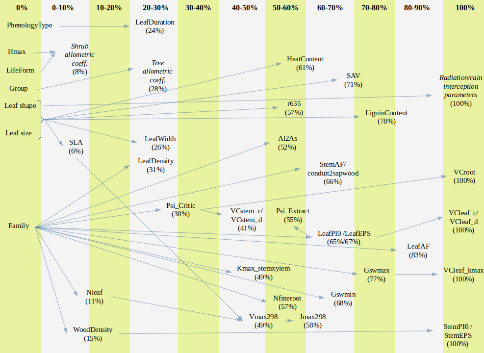
Representation of imputation relationships between model parameters. The percentage of missing parameter values increases from left to right. Left-most parameters are strict.

Figure A.1: Representation of imputation relationships between model parameters. The percentage of missing parameter values increases from left to right. Left-most parameters are strict.

A.3.2 Rooting depth

Parameter \(Z_{95}\) is a strict parameter, but \(Z_{50}\) and \(Z_{100}\) can be imputed when missing, using the following formulae: \[\begin{eqnarray} Z_{50} &=& \exp(\log(Z_{95})/1.4) \\ Z_{100} &=& \exp(\log(Z_{95})/0.95) \end{eqnarray}\]

Note that \(Z_{100}\) will be imputed only if truncateRootDistribution = TRUE in the control parameters.

A.3.3 Shrub allometric coefficients

Missing shrub allometric coefficients are filled using information from Raunkiaer’s life form and maximum plant height (\(H_{max}\)).

Life form	\(H_{max}\)	\(a_{ash}\)	\(b_{ash}\)	\(a_{bsh}\)	\(b_{bsh}\)	\(cr\)
Chamaephyte	[any]	24.5888	1.1662	0.7963	0.3762	0.8076
Phanerophyte	< 300 cm	1.0083	1.8700	0.7900	0.6942	0.6630
Phanerophyte	> 300 cm	5.8458	1.4944	0.3596	0.7138	0.7190
(Hemi)cryptophyte	[any]	24.5888	1.1662	0.7963	0.3762	0.9500

Allometric coefficients were taken from De Cáceres et al. (2019).

A.3.4 Tree allometric coefficients

Missing tree allometric coefficients are replaced with values depending on whether the plant species is a gymnosperm or an angiosperm:

Parameter	Gymnosperm	Angiosperm
\(a_{fbt}\)	0.1300	0.0527
\(b_{fbt}\)	1.2285	1.5782
\(c_{fbt}\)	-0.0147	-0.0066
\(a_{cw}\)	0.747	0.839
\(b_{cw}\)	0.672	0.735
\(a_{cr}\)	1.995	1.506
\(b_{1cr}\)	-0.649	-0.706
\(b_{2cr}\)	-0.020	-0.078
\(b_{3cr}\)	-0.00012	0.00018
\(c_{1cr}\)	-0.004	-0.007
\(c_{2cr}\)	-0.159	0.000
\(fHD_{min}\)	80	40
\(fHD_{max}\)	120	140

A.3.5 Leaf width, specific leaf area and fine foliar ratio

Leaf width (\(LW\)), specific leaf area (\(SLA\)) and the ratio between the weight of leaves plus branches and the weight of leaves alone for branches of 6.35 mm (\(r_{6.35}\)) are key anatomical parameters. When missing from species parameter table, default estimates for these parameters are obtained from combinations of leaf shape and leaf size:

Leaf shape	Leaf size	\(SLA\)	\(LW\)	\(r_{6.35}\)
Broad	Large	16.039	6.898	2.278
Broad	Medium	11.499	3.054	2.359
Broad	Small	9.540	0.644	3.026
Linear	Large	5.522	0.639	3.261
Linear	Medium	4.144	0.639	3.261
Linear	Small	13.189	0.639	3.261
Needle	[any]	9.024	0.379	1.716
Spines	[any]	9.024	0.379	1.716
Scale	[any]	4.544	0.101	1.483

These estimates have been obtained by averaging species-level values across combinations of the categorical variables.

A.3.6 Tissue density

Imputation of the dry weight density of leaves, wood and fine roots (in \(g \cdot cm^{-3}\)) is first performed at the genus level using the corresponding row of SpParams. When genus-level averages are also missing, imputation is performed using taxonomic family (internal data set medfate:::trait_family_means). The percentage of species-level explained variance of these imputations is reported in the following table:

Table A.1: Number of species with available data and percentage of variance explained individually by family and genus, and total explained variance for taxonomically-based imputations of leaf density, wood density and fine root density.
Trait	spp.	Family (%)	Genus (%)	Total (%)
LeafDensity	4258	14.89	28.98	43.9
WoodDensity	14682	23.24	50.82	74.1
FineRootDensity	1490	8.76	32.86	41.6

If the family is not any of those in the table, default values are \(\rho_{leaf} = 0.7\) and \(\rho_{wood} = 0.652\) and \(\rho_{fineroot} = 0.165\).

A.3.7 Specific root length and root length density

Imputation of specific fine root length and fine root length density is first performed at the genus level using the corresponding row of SpParams. When genus-level averages are also missing, imputation of specific fine root length is performed using taxonomic family (internal data set medfate:::trait_family_means). The percentage of species-level explained variance of these imputations is reported in the following table:

Table A.2: Number of species with available data and percentage of variance explained individually by family and genus, and total explained variance for taxonomically-based imputations of specific fine root length.
Trait	spp.	Family (%)	Genus (%)	Total (%)
SRL	2093	8.48	25.87	34.3

Default value for specific fine root length is \(3870\, cm \cdot g^{-1}\). Fine root length density is imputed a value \(10\, cm \cdot cm^{-3}\) when missing at the genus level.

A.3.8 Huber value and ratio of conduits to sapwood

Imputation of the Al2As, the inverse of the Huber value (\(1/Hv\)) and the fraction of sapwood area corresponding to xylem conduits (conduit2sapwood; \(f_{conduits}\)) is first performed at the genus level using the corresponding row of SpParams. When genus-level averages are also missing, imputation is performed using taxonomic family (internal data set medfate:::trait_family_means). The percentage of species-level explained variance of these imputations is reported in the following table:

Table A.3: Number of species with available data and percentage of variance explained individually by family and genus, and total explained variance for taxonomically-based imputations of leaf area to sapwood area and fraction of sapwood corresponding to xylem elements.
Trait	spp.	Family (%)	Genus (%)	Total (%)
conduit2sapwood	651	28.14	42.64	70.8
Al2As	1330	6.66	54.69	61.4

If there is no information derived from taxonomic family for Al2As, a default value is given depending on leaf shape and leaf size:

Leaf shape	Leaf size	`Al2As`
Broad	Large	4768.7
Broad	Medium	2446.1
Broad	Small	2284.9
Linear	Large	2156.0
Linear	Medium	2156.0
Linear	Small	2156.0
Needle	[any]	2751.7
Scale	[any]	1696.6

Missing values for \(f_{conduits}\), the fraction of sapwood corresponding to conduits are derived from taxonomic family (see table above). If information from taxonomic family is missing, default values are \(f_{conduits} = 0.7\) (i.e. 30% of parenchyma) for angiosperms, and \(f_{conduits} = 0.925\) (i.e. 7.5% of parenchyma) for gymnosperms (Plavcová & Jansen 2015).

A.3.9 Fine root to leaf area ratio

When missing, the fine root area to leaf area ratio is given a default value of \(RLR = 1\; m^2\cdot m^{-2}\).

A.3.10 Leaf phenology

When missing, leaf duration is assigned a value of 1 year for winter-deciduous species and 2.41 years for the remaining leaf phenology types.

Default values for leaf phenological parameters are the same regardless of the leaf phenology type:

Phenology type	`t0gdd`	`Sgdd`	`Ssen`	`Phsen`	`Tbsen`	`xsen`	`ysen`
One-flush evergreen	50	200	8268	12.5	28.5	2	2
Winter deciduous	50	200	8268	12.5	28.5	2	2
Winter semi-deciduous	50	200	8268	12.5	28.5	2	2
Drought deciduous	50	200	8268	12.5	28.5	2	2

Leaf senescence values were derived for deciduous broad-leaved forests by Delpierre et al. (2009).

A.3.11 Basic transpiration and water-use efficiency

When the basic soil water balance model is used, \(T_{max,LAI}\) and \(T_{max,sqLAI}\) are species-specific parameters that regulate the maximum transpiration of plant cohorts (see 6.1.1). When these parameters are missing from SpParams table, they are given default values \(T_{max,LAI} = 0.134\) and \(T_{max,sqLAI} = -0.006\), according to Granier et al. (1999).

When maximum water use efficiency (\(WUE_{\max}\)) is missing, it is given a value of \(WUE_{\max} = 7.55\). By default, the coefficient describing the decay of water use efficiency with lower light levels is given a default value of \(WUE_{PAR} = 0.2812\), and the coefficient regulating the relationship between gross photosynthesis and CO2 concentration is given a default \(WUE_{CO2} = 0.0028\).

When missing, the water potential corresponding to 50% of transpiration (\(\Psi_{extract}\)) is estimated by calculating the water potential corresponding to the loss leaf turgor (\(\Psi_{tlp}\)), using equation (10.4) from Bartlett et al. (2012). The parameters of the leaf pressure-volume curve needed for applying equation (10.4) may be themselves estimated (see A.3.14). Note that \(\Psi_{tlp}\) has been found to be highly correlated to \(\Psi_{gs50}\), the water potential corresponding to 50% of stomatal conductance (Bartlett et al. 2016).

A.3.12 Radiation balance and water interception

Default value for direct light extinction is \(k_b = 0.8\). Default values for diffuse radiation extinction, absorbance, reflectance and water interception parameters depend on the leaf shape:

Leaf shape	\(k_{PAR}\)	\(\alpha_{SWR}\)	\(\gamma_{SWR}\)	\(s_{water}\)
Broad	0.55	0.70	0.18	0.5
Linear	0.45	0.70	0.15	0.8
Needle/Scale	0.50	0.70	0.14	1.0

where \(k_{PAR}\) is the diffuse PAR extinction coefficient, \(\alpha_{SWR}\) is the short-wave radiation leaf absorbance coefficient, \(\gamma_{SWR}\) is the short-wave radiation leaf reflectance (albedo) and \(s_{water}\) is the crown water storage capacity per LAI unit.

A.3.13 Stomatal conductance

Imputation of the minimum and maximum conductance to water vapour (\(g_{swmin}\) and \(g_{swmax}\); in \(mol\, H_2O \cdot s^{-1} \cdot m^{-2}\)) is first performed at the genus level using the corresponding row of SpParams. When genus-level averages are also missing, imputation is performed using taxonomic family (internal data set medfate:::trait_family_means). The percentage of species-level explained variance of these imputations is reported in the following table.

Table A.4: Number of species with available data and percentage of variance explained individually by family and genus, and total explained variance for taxonomically-based imputations of minimum and maximum conductance to water vapour.
Trait	spp.	Family (%)	Genus (%)	Total (%)
Gswmin	465	-6.34	82.84	76.5
Gswmax	536	3.79	-4.78	-1.0

If there is no information derived from taxonomic family, \(g_{swmin} = 0.0049\) and \(g_{swmax} = 0.200\).

A.3.14 Pressure-volume curves

Parameters of the pressure-volume curve (i.e. \(\pi_{0,stem}\) and \(\epsilon_{stem}\)) for leaf and stem symplastic tissue are required for each species.

When parameters for stem tissue are missing, medfate estimates them from wood density following Christoffersen et al. (2016): \[\begin{equation} \pi_{0,stem} = 0.52 - 4.16 \cdot \rho_{wood} \end{equation}\]

\[\begin{equation} \epsilon_{stem} = \sqrt{1.02 \cdot e^{8.5\cdot \rho_{wood}}-2.89} \end{equation}\] while the apoplastic fraction of stem is assumed \(f_{apo,stem} = f_{conduits}\) (see A.3.8).

Imputation of leaf pressure-volume parameters, i.e. \(\pi_{0,leaf}\) (LeafPI0), \(\epsilon_{leaf}\) (LeafEPS) and \(f_{apo,leaf}\) (LeafAF), is first performed at the genus level using the corresponding row of SpParams. When genus-level averages are also missing, imputation is performed using taxonomic family (internal data set medfate:::trait_family_means). The percentage of species-level explained variance of these imputations is reported in the following table.

Table A.5: Number of species with available data and percentage of variance explained individually by family and genus, and total explained variance for taxonomically-based imputations of leaf pressure-volume parameters.
Trait	spp.	Family (%)	Genus (%)	Total (%)
LeafPI0	550	7.03	20.75	27.8
LeafEPS	367	16.45	37.95	54.4
LeafAF	118	18.22	26.19	44.4

If family-level values are missing, following Bartlett et al. (2012) average values for Mediterranean climate leaves are taken as defaults, i.e. \(\pi_{0,leaf} = -2\) MPa, \(\epsilon_{leaf} = 17\), whereas a 29% leaf apoplastic fraction is assumed (i.e. \(f_{apo,leaf} = 0.29\)).

A.3.15 Stem and root maximum hydraulic conductivity

Tissue-level maximum conductivity parameters (i.e. \(K_{stem,max,ref}\) and \(K_{root,max,ref}\)) are not direct parameters to simulation functions. Instead, they are scaled to estimate stem- and root-level hydraulic conductances (i.e. \(k_{stem, \max}\) and \(k_{root, \max}\)) using plant size (see A.4.1 and A.4.3 for details). \(K_{stem,max,ref}\) and \(K_{root,max,ref}\) are supplied via species parameter table and missing values can therefore occur.

Imputation of \(K_{stem,max,ref}\) (Ks or Kmax_stemxylem) is first performed at the genus level using the corresponding row of SpParams. When genus-level averages are also missing, imputation is performed using taxonomic family (internal data set medfate:::trait_family_means). The percentage of species-level explained variance of these imputations is reported in the following table.

Table A.6: Number of species with available data and percentage of variance explained individually by family and genus, and total explained variance for taxonomically-based imputations of maximum stem hydraulic conductivity.
Trait	spp.	Family (%)	Genus (%)	Total (%)
Ks	1965	3.28	66.19	69.5

If family-level values are missing, suitable \(K_{stem,max,ref}\) values are decided according to combinations of taxon group (either Angiosperm or Gymnosperm), growth form (either tree or shrub) and leaf phenology (Maherali et al. 2004):

Group	Growth form	Leaf phenology	\(K_{stem,max,ref}\)
Angiosperm	Tree	Winter-(semi)deciduous	1.58
Angiosperm	Shrub	Winter-(semi)deciduous	1.55
Angiosperm	Tree/Shrub	Evergreen	2.43
Gymnosperm	Tree	any	0.48
Gymnosperm	Shrub	any	0.24

Following Oliveras et al. (2003), missing values for \(K_{root,max,ref}\) are assumed to be four-times the values given or estimated for \(K_{stem,max,ref}\).

A.3.16 Leaf maximum hydraulic conductance

Leaf maximum hydraulic conductance (\(k_{l, max}\), in \(mmol \cdot m^{-2} \cdot s^{-1} \cdot MPa^{-1}\)) is an input parameter that should be provided for each species. When missing, leaf maximum hydraulic conductance can be estimated from maximum stomatal conductance (\(g_{swmax}\)), following Franks (2006) (original coefficients were modified for better fit): \[\begin{equation} k_{l, max} = (g_{swmax}/0.015)^{1/1.3} \end{equation}\] Note that values for \(g_{swmax}\) may also be imputed (see A.3.13).

A.3.17 Xylem vulnerability

Stem vulnerability

Imputation of \(\Psi_{50,stem}\) is first performed at the genus level using the corresponding row of SpParams. When genus-level averages are also missing, imputation is performed using taxonomic family (internal data set medfate:::trait_family_means). The percentage of species-level explained variance of these imputations is reported in the following table.

Table A.7: Number of species with available data and percentage of variance explained individually by family and genus, and total explained variance for taxonomically-based imputations of stem P50.
Trait	spp.	Family (%)	Genus (%)	Total (%)
VCstem_P50	1916	18.7	40.1	58.8

If family-level values is missing, a suitable estimate of \(\Psi_{50,stem}\) the water potential corresponding to 50% of conductance loss, can be obtained from Maherali et al. (2004) according to combinations of taxon group (either Angiosperm or Gymnosperm), growth form (either tree or shrub) and leaf phenology:

Group	Growth form	Leaf phenology	\(\Psi_{50,stem}\)
Angiosperm	Tree/Shrub	Winter-(semi)deciduous	-2.34
Angiosperm	Tree	Evergreen	-1.51
Angiosperm	Shrub	Evergreen	-5.09
Gymnosperm	Tree	any	-4.17
Gymnosperm	Shrub	any	-8.95

\(\Psi_{50,stem}\) estimates are taken for parameter \(\Psi_{critic}\), in the case of the basic water balance model.

Water potentials corresponding to 12% and 88% PLC (\(\Psi_{12,stem}\) and \(\Psi_{88,stem}\)), when missing are not estimated using genus-level averages, in order to avoid inconsistencies in the stem vulnerability curve (i.e., with respect to \(\Psi_{50,stem}\)). When \(\Psi_{88,stem}\) is missing, a regression equation is used to estimate it from \(\Psi_{50,stem}\) (\(R^2_{adj} = 0.633\); data compiled using forestables): \[\begin{equation} \Psi_{88,stem} = 1.43637 \cdot \Psi_{50,stem} \end{equation}\]

Similarly, when \(\Psi_{12,stem}\) is missing, a similar regression equation is used to estimate it from \(\Psi_{50,stem}\) (\(R^2_{adj} = 0.724\); data compiled using forestables): \[\begin{equation} \Psi_{12,stem} = 0.626191 \cdot \Psi_{50,stem} \end{equation}\]

Finally, estimates of the Weibull function (\(c_{stem}\) and \(d_{stem}\)) are obtained from \(\Psi_{50,stem}\) and \(\Psi_{88,stem}\) via function hydraulics_psi2Weibull().

Root vulnerability

Imputation of \(\Psi_{50,stem}\) is first performed at the genus level using the corresponding row of SpParams. The percentage of species-level explained variance of imputations using genus averages is reported in the following table.

Table A.8: Number of species with available data and percentage of variance explained individually by family and genus, and total explained variance for taxonomically-based imputations of root P50.
Trait	spp.	Family (%)	Genus (%)	Total (%)
VCroot_P50	137	22.39	44.92	67.3

Note that vulnerability curves for root xylem are less common than for stem xylem. If genus-level averages are missing, a linear relationship is used to estimate \(\Psi_{50, root}\) from \(\Psi_{50,stem}\) (\(R^2_{adj} = 0.499\); data compiled using forestables): \[\begin{equation} \Psi_{50, root} = 0.627 \cdot \Psi_{50,stem} \end{equation}\] Finally, \(\Psi_{88,stem}\) and the Weibull vulnerability parameters are obtained as explained for stems.

Water potentials corresponding to 12% and 88% root PLC (\(\Psi_{12,root}\) and \(\Psi_{88,root}\)), when missing are not estimated using genus-level averages, in order to avoid inconsistencies in the root vulnerability curve (i.e., with respect to \(\Psi_{50,root}\)). Similarly to the stem vulnerability curve, when \(\Psi_{88,root}\) is missing, a regression equation is used to estimate it from \(\Psi_{50,root}\) (\(R^2_{adj} = 0.742\); data compiled using forestables): \[\begin{equation} \Psi_{88,root} = 1.57274 \cdot \Psi_{50,root} \end{equation}\]

Similarly, when \(\Psi_{12,root}\) is missing, a similar regression equation is used to estimate it from \(\Psi_{50,root}\) (\(R^2_{adj} = 0.804\)): \[\begin{equation} \Psi_{12,root} = 0.52103 \cdot \Psi_{50,root} \end{equation}\]

Finally, estimates of the Weibull function (\(c_{root}\) and \(d_{root}\)) are obtained from \(\Psi_{50,root}\) and \(\Psi_{88,root}\) via function hydraulics_psi2Weibull().

Leaf vulnerability

Imputation of \(\Psi_{50,leaf}\) is first performed at the genus level using the corresponding row of SpParams. The percentage of species-level explained variance of imputations using genus averages is reported in the following table.

Table A.9: Number of species with available data and percentage of variance explained individually by family and genus, and total explained variance for taxonomically-based imputations of leaf P50.
Trait	spp.	Family (%)	Genus (%)	Total (%)
VCleaf_P50	634	10.37	39.65	50

Vulnerability curves for leaf xylem are also less common than for stem xylem. If genus-level averages values are missing, a relationship calibrated with data from Bartlett et al. (2016) is used to estimate \(\Psi_{50, leaf}\) from the water potential at turgor loss point (\(\Psi_{tlp}\)): \[\begin{equation} \Psi_{50, leaf} = 0.2486 + 0.9944 \cdot \Psi_{tlp} \end{equation}\]

Water potentials corresponding to 12% and 88% leaf PLC (\(\Psi_{12,leaf}\) and \(\Psi_{88,leaf}\)), when missing are not estimated using genus-level averages, in order to avoid inconsistencies in the leaf vulnerability curve (i.e., with respect to \(\Psi_{50,leaf}\)). Similarly to the stem vulnerability curve, when \(\Psi_{88,leaf}\) is missing, a regression equation is used to estimate it from \(\Psi_{50,leaf}\) (\(R^2_{adj} = 0.765\); data compiled using forestables): \[\begin{equation} \Psi_{88,leaf} = 1.28837 \cdot \Psi_{50,leaf} \end{equation}\]

Similarly, when \(\Psi_{12,leaf}\) is missing, a similar regression equation is used to estimate it from \(\Psi_{50,leaf}\) (\(R^2_{adj} = 0.766\)): \[\begin{equation} \Psi_{12,leaf} = 0.76389 \cdot \Psi_{50,leaf} \end{equation}\]

Finally, estimates of the Weibull function (\(c_{leaf}\) and \(d_{leaf}\)) are obtained from \(\Psi_{50,leaf}\) and \(\Psi_{88,leaf}\) via function hydraulics_psi2Weibull().

A.3.18 Photosynthesis rates

Rubisco’s maximum carboxylation rate at 25ºC (\(V_{max, 298}\), in \(\mu mol CO_2 \cdot s^{-1} \cdot m^{-2}\)) is a required input parameter for each species (Vmax298). When missing, the work by Walker et al. (2014) suggests that suitable estimates can be derived from \(SLA\) and \(N_{area}\), the latter being the nitrogen concentration per leaf area: \[\begin{equation} V_{max, 298} = e^{1.993 + 2.555\cdot \log(N_{area}) - 0.372 \cdot \log(SLA) + 0.422 \cdot \log(N_{area})\cdot \log(SLA) } \end{equation}\]

In turn, imputation for \(SLA\) is explained in A.3.5, whereas values for \(N_{area}\) are determined from \(N_{leaf}\) and \(SLA\), being \(N_{leaf}\) estimated as indicated in A.3.19. Would \(N_{leaf}\) and \(SLA\) values be both unavailable, a default value of 100 \(\mu mol CO_2 \cdot s^{-1} \cdot m^{-2}\) is used for \(V_{max, 298}\) imputation.

When the maximum rate of electron transport at the same temperature (\(J_{max, 298}\)) is not provided by the user, it can be estimated from \(V_{max, 298}\) using (Walker et al. 2014):

\[\begin{equation} J_{max, 298} = e^{1.197 + 0.847\cdot \log(V_{max,298})} \end{equation}\]

A.3.19 Maintenance respiration rates

Imputation of maintenance respiration rates for leaves, sapwood and fine roots (\(RER_{leaf}\), \(RER_{sapwood}\) and \(RER_{fineroot}\); all in \(g\,gluc\cdot g\,dry^{-1}\cdot day^{-1}\)) is first performed at the genus level using the corresponding row of SpParams. When missing at the genus, they are estimated from corresponding tissue nitrogen concentrations (\(N_{leaf}\), \(N_{sapwood}\) and \(N_{fineroot}\); all in \(mg\,N \cdot g\,dry^{-1}\)) following the equations given by Reich et al. (2008) (after appropriate unit conversion): \[\begin{eqnarray} RER_{leaf} &=& e^{0.691+ 1.639 \cdot \log(N_{leaf}))} \\ RER_{sapwood} &=& e^{1.024 + 1.344 \cdot \log(N_{sapwood}))} \\ RER_{fineroot} &=& e^{0.980 + 1.352 \cdot \log(N_{fineroot}))} \end{eqnarray}\] where in the previous equations nitrogen concentrations are in \(mmol\,N\cdot g\,dry^{-1}\) and respiration rates in \(nmol\,CO2\cdot g\,dry^{-1}\cdot s^{-1}\).

In turn, imputation of tissue nitrogen concentration is first performed at the genus level using the corresponding row of SpParams. When genus-level averages are also missing, imputation is performed using taxonomic family (internal data set medfate:::trait_family_means). The percentage of species-level explained variance of these imputations is reported in the following table.

Table A.10: Number of species with available data and percentage of variance explained individually by family and genus, and total explained variance for taxonomically-based imputations of tissue nitrogen concentration.
Trait	spp.	Family (%)	Genus (%)	Total (%)
Nleaf	11920	17.43	38.78	56.2
Nsapwood	65	34.11	16.79	50.9
Nfineroot	1793	12.57	39.50	52.1

When family values are also missing, default tissue-averaged nitrogen concentrations are given: \(N_{leaf} = 20.088\), \(N_{sapwood} = 3.9791\) and \(N_{fineroot} = 12.207\).

Default control values (\(MR_{leaf} = 0.00260274\)), sapwood (\(MR_{sapwood} = 6.849315e-05\)) and fine roots (\(MR_{fineroot} 0.002054795\)) were used in previous model versions, derived from Ogle & Pacala (2009), but these are no longer used because of easier parameterization using tissue nitrogen concentration.

A.3.20 Relative growth rates

When missing at the species parameter table, maximum relative growth rates for leaves, sapwood and fine roots are taken from control parameters. Default values are provided in 15.5.3.

A.3.21 Senescence rates

When missing at the species parameter table, senescence rates for sapwood and fine roots are taken from control parameters. The default daily senescence rate for fine roots is \(0.001897231\, day^{-1}\) which corresponds to a 50% annual turnover rate (Gill & Jackson 2000).

A.3.22 Relative starch for sapwood growth

When missing at the species parameter table, the minimum relative starch for sapwood growth is taken from control parameters. Default value is provided in 15.5.3.

A.3.23 Wood carbon

Imputation of \(C_{wood}\) is first performed at the genus level using the corresponding row of SpParams. When genus-level averages are also missing, imputation is performed using taxonomic family (internal data set medfate:::trait_family_means). The percentage of species-level explained variance of these imputations is reported in the following table.

Table A.11: Number of species with available data and percentage of variance explained individually by family and genus, and total explained variance for taxonomically-based imputations of wood carbon content.
Trait	spp.	Family (%)	Genus (%)	Total (%)
WoodC	614	17.91	27.76	45.7

If family-level values are also missing, default value of \(C_{wood} = 0.5\,g\,C\cdot g\,dry^{-1}\) is used.

A.3.24 Mortality baseline rate

When missing at the species parameter table, the mortality baseline rate is taken from control parameters. Default value is provided in 15.5.3.

A.3.25 Recruitment

Imputation of missing values for recruitment is specified via control parameters. Default values are provided in 19.4.3.

A.3.26 Flammability

Default values for the surface-area-to-volume ratio (\(\sigma\)), fuel heat content (\(h\)) and lignin percent (\(LI\)) are defined from leaf size and leaf shape as follows:

Leaf shape	Leaf size	\(\sigma\)	\(h\)	\(LI\)
Broad	Large	5740	19740	15.50
Broad	Medium	4039	19825	20.21
Broad	Small	4386	20062	22.32
Linear/Needle	Large	3620	18250	24.52
Linear/Needle	Medium	4758	21182	24.52
Linear/Needle	Small	6697	21888	18.55
Spines	[any]	6750	20433	14.55
Scale	[any]	1120	20504	14.55

Default value for the density of fuel particles (\(\rho_p\)) is 400 \(kg\cdot m^{-3}\).

A.4 Scaling size-related parameters

A.4.1 Stem xylem maximum conductance

Estimation of maximum stem conductance (\(k_{s,max}\), in \(mmol \cdot m^{-2} \cdot s^{-1} \cdot MPa^{-1}\)) is done by function hydraulics_maximumStemHydraulicConductance() and follows the work by Savage et al. (2010), Olson et al. (2014) and Christoffersen et al. (2016). Calculations are based on tree height and two species-specific parameters: maximum sapwood reference conductivity (\(K_{s,max,ref}\)) and the ratio of leaf area to sapwood area (\(A_{l}/A_{s}\); Al2As in SpParamsMED), i.e. the inverse of the Huber value \(H_v\).

The reference value for maximum sapwood conductivity \(K_{s,max,ref}\) is assumed to have been measured on a terminal branch of a plant of known height \(H_{ref}\). If our target plant is very different in height, the conduits of terminal branches will have different radius and hence conductivity. We correct the reference conductivity to the target plant height using the following empirical relationship, developed by Olson et al. (2014) between tree height and diameter of conduits for angiosperms and the equation described by Christoffersen et al. (2016): \[\begin{eqnarray} 2 \cdot r_{int,H}&=& 10^{1.257+(0.24\cdot log_{10}(H))} \\ 2 \cdot r_{int,ref}&=&10^{1.257+(0.24\cdot log_{10}(H_{ref}))}\\ K_{s,max,cor}&=&K_{s,max,ref}\cdot (r_{int,H}/r_{int,ref})^{2} \end{eqnarray}\] Where \(r_{int,H}\) is the radius of conduits for a terminal branch of a tree of height \(H\) and \(r_{int,ref}\) is the corresponding radius for a tree of height \(H_{ref}\) (\(H\) and \(H_{ref}\) are measured in m). The form of the empirical relationship by Olson et al. (2014) is:

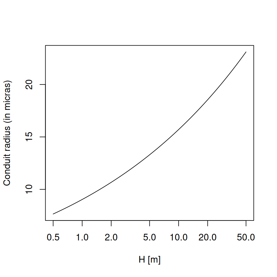
Let’s consider an example for a Quercus ilex target tree of 4m height and where species-specific conductivity \(K_{s,max,ref} = 0.77\) is the apical value for trees of \(H_{ref} = 6.6\) m (in , values of \(H_{ref}\) are taken from median height values; see parameter Hmed in SpParamsMED). The corrected conductivity for a tree of height 4 m will be a bit lower than that of the reference height:

xylem_kmax = 0.77
H = 400 # in cm
Href = 660 # in cm
f = hydraulics_referenceConductivityHeightFactor(Href, H);
f

## [1] 0.7863352

xylem_kmax_cor = xylem_kmax * f
xylem_kmax_cor

## [1] 0.6054781

Once the reference conductivity is corrected, the maximum stem conductance without accounting for conduit taper is: \[\begin{equation} k_{s,max, notaper}=\frac{1000}{0.018} \frac{K_{s,max,cor}\cdot A_{s}}{H\cdot A_{l}} \end{equation}\] where \(H\) is the tree height (here in m), \(A_{s}\) is the sapwood area, \(A_{l}\) is the leaf area and 1000/0.018 is a factor used to go from kg to mmol. The ratio \(A_{l}/A_{s} = 1/H_v\) is a fixed species parameter in soil water balance calculations (see parameter Al2As), but becomes variable when simulating plant growth. Let’s assume that Quercus ilex the leaf to sapwood area ratio is \(A_{l}/A_{s} = 2512\). The maximum (leaf-specific) stem conductance without taper (\(k_{s, max, notaper}\)) for the tree of 4 m height is then:

Al2As = 2512 

kstemmax = hydraulics_maximumStemHydraulicConductance(xylem_kmax, 
                  Href, Al2As, H, taper = FALSE)
kstemmax

## [1] 3.347698

In order to consider taper of xylem conduits we calculate the whole-tree conductance per unit leaf area (\(k_{s, max, taper}\)) as described in Christoffersen et al. (2016): \[\begin{equation} k_{s, max, taper}=\frac{1000}{0.018} \cdot \frac{K_{s,max,pet}\cdot A_{s}}{H\cdot A_{l}}\cdot \chi_{tap:notap,ag}(H) \end{equation}\] where \(K_{s,max,pet}\) is the conductivity at the petiole level and \(\chi_{tap:notap,ag}(H)\) is the taper factor accounting for the decrease in the xylem conduits diameter with the height, from the petiole to base of the trunk, which mitigates the negative effects of height on the hydraulic safety. The conductivity at the petiole level is obtained from \(K_{s,max,ref}\) using again: \[\begin{equation} K_{s,max,pet} = K_{s,max,ref}\cdot (r_{int, pet}/r_{int,ref})^{2} \end{equation}\] where \(r_{int, pet}\) is the radius of the petiole in the model of Savage et al. (2010). Christoffersen et al. (2016) use \(r_{int, pet} = 10\) \(\mu m\) but we define it as the radius of apical conduits in a tree of 1 m height:

hydraulics_terminalConduitRadius(100.0)

## [1] 9.035871

\(\chi_{tap:notap,ag}(H)\) is calculated as described in the Appendix 1 section of Christoffersen et al. (2016) (see also Savage et al. (2010)). The following figure shows the value of \(\chi_{tap:notap,ag}\) for different heights:

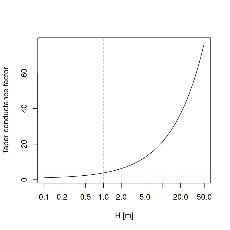
Note that, since \(\chi_{tap:notap,ag}(1) = 3.82\) (indicated using grey dashed lines in the last figure), the equation of maximum conductance with taper would give a higher conductance than the equation without taper for a tree of 1 m height, which is supposed to have a conductance equal to conductivity. To solve this issue we define the taper factor as \(\chi_{tap:notap,ag}(H)/\chi_{tap:notap,ag}(1)\): \[\begin{equation} k_{s, max, taper}=\frac{1000}{0.018} \cdot \frac{K_{s,max,pet}\cdot A_{s}}{H\cdot A_{l}}\cdot \frac{\chi_{tap:notap,ag}(H)}{\chi_{tap:notap,ag}(1)} \end{equation}\] The maximum stem conductance with taper (\(k_{s, max, taper}\)) of a Q. ilex tree of 4 m height, calculated with this second equation, is:

kstemmax_tap = hydraulics_maximumStemHydraulicConductance(xylem_kmax, 
                      Href, Al2As, H, taper = TRUE)
kstemmax_tap

## [1] 4.764396

The next two plots show the variation of \(k_{s,max}\) for Q. ilex depending on the tree height and with/without considering taper of conduits. The plot on the right (both axes in log) show the slope of the dependency of conductance with height in both cases:

A.4.2 Leaf maximum hydraulic conductance

A.4.3 Root xylem maximum hydraulic conductance

To obtain maximum root xylem conductance (\(k_{r, max}\), in \(mmol \cdot m^{-2} \cdot s^{-1} \cdot MPa^{-1}\)), one option taken by Christoffersen et al. (2016) is to assume that minimum stem resistance (inverse of maximum conductance) represents a fixed proportion of the minimum total tree (stem+root) resistance. A value 0.625 (i.e. 62.5%) suggested by these authors leads to maximum total tree conductance for our Q. ilex tree being:

ktot = kstemmax*0.625
ktot

## [1] 2.092311

and the maximum root xylem conductance would be therefore:

krootmax = 1/((1/ktot)-(1/kstemmax))
krootmax

## [1] 5.579497

Now, we need to divide total maximum conductance of the root system xylem among soil layers we need weights inversely proportional to the length of transport distances (Sperry et al. 2017). Vertical transport lengths can be calculated from soil depths and radial spread can be calculated assuming cylinders with volume proportional to the proportions of fine root biomass. Let’s assume a soil with three layers:

s <- soil(defaultSoilParams(3))
d <- s$widths
d

## [1]  300  700 1000

The proportion of fine roots in each layer, assuming a linear dose response model, will be:

Z50 <- 200
Z95 <- 1500
v1 <- root_ldrDistribution(Z50,Z95, NA, d)
v1

##           [,1]      [,2]       [,3]
## [1,] 0.6661036 0.2784153 0.05548106

Having this information, the calculation of root length (i.e. the sum of vertical and radial lengths) to each layer (\(L_j\)) is done using function root_coarseRootLengths():

rfc <- c(20,50,70)
Vol <- root_coarseRootSoilVolumeFromConductance(1.0, 2500,krootmax,
                                               v1, d, rfc)
l <- root_coarseRootLengthsFromVolume(Vol, v1, d, rfc)
l

## [1] 4503.445 3250.363 3085.055

where lengths are in mm. The proportion of total root xylem conductance corresponding to each layer (\(w_j\)) is given by root_xylemConductanceProportions():

w1 <- hydraulics_rootxylemConductanceProportions(v1, l)
w1

## [1] 0.09131268 0.15767645 0.75101087

Xylem conductance proportions can be quite different than the fine root biomass proportions. This is because radial lengths are largest for the first top layers and vertical lengths are largest for the bottom layers. The maximum root xylem conductances of each layer will be the product of maximum total conductance of root xylem and weights:

w1*krootmax

## [1] 0.5094788 0.8797553 4.1902629

The maximum root xylem conductances of each layer would be:

krootmaxvec = w1*krootmax
krootmaxvec

## [1] 0.5094788 0.8797553 4.1902629

and the fraction of total xylem resistance due to stem would be:

(1/kstemmax)/((1/kstemmax)+(1/krootmax))

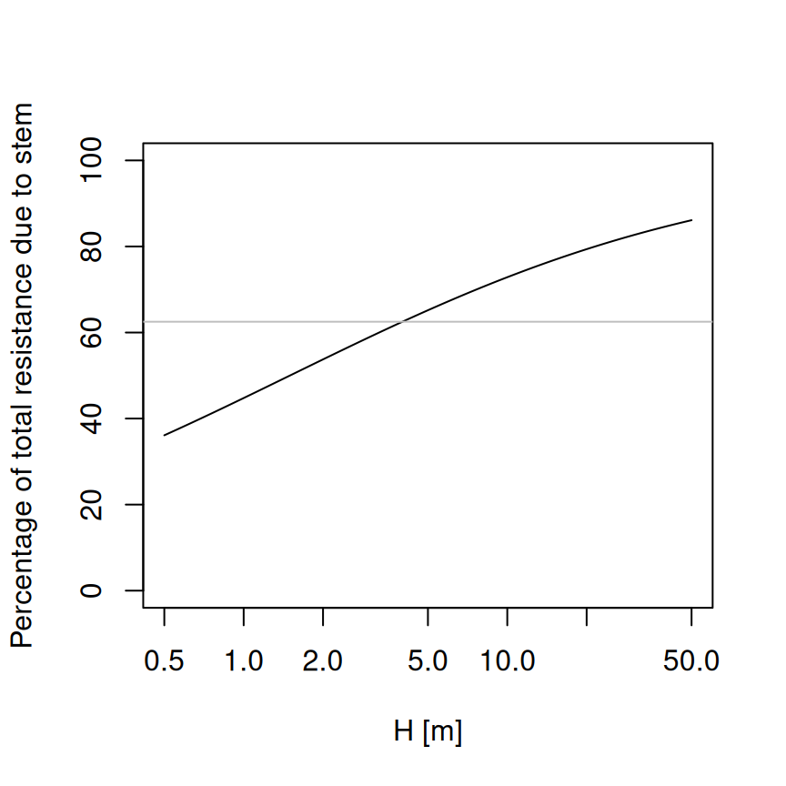
## [1] 0.625

In contrast with the approach of Christoffersen et al. (2016), in this approach the root maximum conductance depends root length and distribution, and is not a fixed fraction of stem maximum conductance. Assuming constant root length, then the proportion of total resistance due to the stem will increase with tree height (Magnani et al. 2000):

where the horizontal gray line indicates the value of 62.5%. Of course rooting depth also increases with tree age, but young trees have higher root-to-shoot ratios than older ones. Hence, a root maximum conductance that is not fixed but increases with age seems a priori more realistic. Moreover, Christoffersen et al. (2016) justify the value of 62.5% from a study which quantified total aboveground and belowground resistance in tropical trees (Fisher et al. 2006) under near-saturated (wet season) conditions, but values of belowground resistance reported in this study for wet conditions and trees of 30 m height are around 13%, which equals to 87% fraction of aboveground resistance. On the other hand, while rooting depths are limited by soil depth, lateral root length increases with age and, hence, the model could be made more realistic if this is taken into account and the curve above would probably saturate at lower percentages.

A.4.4 Rhizosphere maximum hydraulic conductance

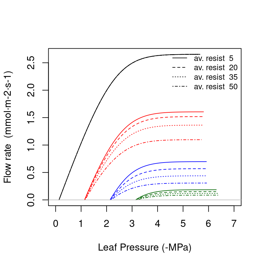
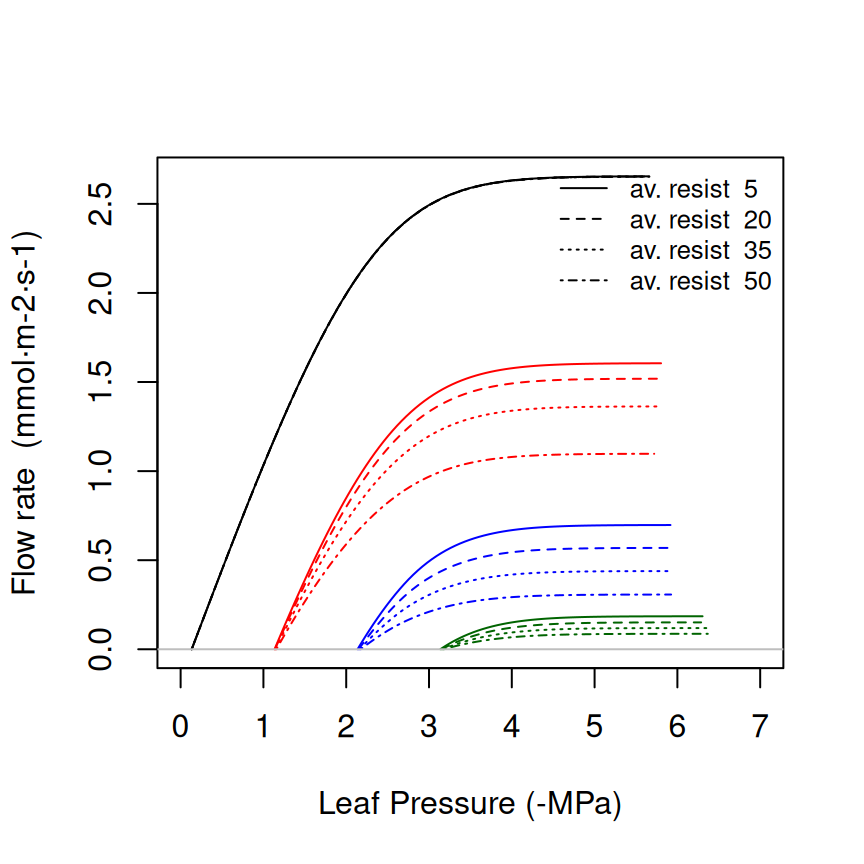
Maximum rhizosphere conductance (\(k_{rh, max}\), in \(mmol \cdot m^{-2} \cdot s^{-1} \cdot MPa^{-1}\)) is difficult to measure directly, as it depends on the rhizosphere (i.e. fine root) surface in each soil layer, and will probably always be a parameter to be calibrated. Instead of trying to estimate rhizosphere surface from root architecture (Sperry et al. 1998), we follow Sperry et al. (2016) and determine the maximum rhizosphere conductance in each layer from an inputed ‘average percentage rhizosphere resistance’. The percentage of continuum resistance corresponding to the rhizosphere is calculated from the vulnerability curves of stem, root and rhizosphere at the same water potential. The average resistance is found by evaluating the percentage for water potential values between 0 and \(\Psi_{crit}\). The following figure illustrates how the supply function, for different soil water potentials, is affected by increasing values of the average percentage of rhizosphere resistance:

Sperry et al. (2016) found average percentages of rhizosphere resistance around 67%, but these exceptionally-high values were probably a consequence of using an unsegmented supply function (i.e. single vulnerability curve for roots, stem and leaves). If we specify a 15% of average resistance in the rhizosphere (see parameter averageFracRhizosphereResistance in function defaultControl()), the maximum rhizosphere conductance values for the three layers are found calling:

krmax = rep(0,3) 
krmax[1]= hydraulics_findRhizosphereMaximumConductance(15, 
                     s$VG_n[1],s$VG_alpha[1],
                     krootmax, rootc,rootd, 
                     kstemmax, stemc, stemd,
                     kleafmax, leafc, leafd, 0)
krmax[2] = hydraulics_findRhizosphereMaximumConductance(15, 
                      s$VG_n[2],s$VG_alpha[2],
                      krootmax, rootc,rootd, 
                      kstemmax, stemc, stemd,
                      kleafmax, leafc, leafd, 0)
krmax[3] = hydraulics_findRhizosphereMaximumConductance(15, 
                      s$VG_n[3],s$VG_alpha[3],
                      krootmax, rootc,rootd, 
                      kstemmax, stemc, stemd,
                      kleafmax, leafc, leafd, 0)
krmax

## [1] 85636744 85636744 85636744

The values are the same because the texture of the three layers is the same in this case. If we take into account root distribution, actual maximum rhizosphere conductance values are:

krmax*v1

##          [,1]     [,2]    [,3]
## [1,] 57042945 23842581 4751218

A.4.5 Plant water storage capacity

The water storage capacity of sapwood tissue per leaf area unit (\(V_{sapwood}\); in \(l \cdot m^{-2}\)) can be estimated as the product of stem height (\(H\) in m) and Huber value (\(H_v\); ratio of sapwood area to leaf area in \(m^2 \cdot m^{-2}\)) times a factor to account for the non-cylindrical shape (http://www.fao.org/forestry/17109/en/): \[\begin{equation} V_{sapwood} = 10^3 \cdot 0.48 \cdot H \cdot H_v \cdot \Theta_{sapwood} \end{equation}\] \(\Theta_{sapwood}\) is sapwood porosity (\(cm^3\) of water per \(cm^3\) of sapwood tissue), which can be estimated from wood density (\(\rho_{wood}\); in \(g \cdot cm^{-3}\)): \[\begin{equation} \Theta_{sapwood} = 1 - (\rho_{wood} / 1.54) \end{equation}\] where the density of wood substance can be assumed to be fixed and equal to 1.54 \(g \cdot cm^{-3}\) (Dunlap 1914). For example, wood densities ranging from 0.443 to 1.000 \(g \cdot cm^{-3}\) result in sapwood porosity values between 0.35 and 0.71.

Water storage capacity of leaf tissue per leaf area unit (\(V_{leaf}\); in \(l \cdot m^{-2}\)) can be estimated as the product of specific leaf area (SLA; in \(m^2 \cdot kg^{-1}\)) and leaf density (\(\rho_{leaf}\); in \(g \cdot cm^{-3}\)): \[\begin{equation} V_{leaf} = \frac{1}{SLA \cdot \rho_{leaf}} \cdot \Theta_{leaf} \end{equation}\] \(\Theta_{leaf}\) is leaf porosity (\(cm^3\) of water per \(cm^3\) of leaf tissue), which can be estimated from leaf density: \[\begin{equation} \Theta_{leaf} = 1 - (\rho_{leaf} / 1.54) \end{equation}\] where the density of wood substance can be assumed to be fixed and equal to 1.54 \(g \cdot cm^{-3}\) (Dunlap 1914).

For example, let’s calculate the stem and leaf water capacity for a Q. ilex tree of 15 m height:

ld = 0.7
SLA = 5.870 
moisture_leafWaterCapacity(SLA, ld)

## [1] 0.1327463

A.4.6 Horizontal root overlap

A.4.6.1 Basic water balance

A given plant cohort \(i\) will have its roots in layer \(s\) partitioned among different water pools. We thus need to define \(fr_{i,s,j}\), the (horizontal) proportion of fine roots of cohort \(i\) in layer \(s\) of the water pool \(j\), with the restriction that: \[\begin{equation} \sum_{j}{fr_{i,s,j}} = 1 \,\, \forall i,s \end{equation}\] It is important to realize that proper estimation of \(fr_{i,s,j}\) is challenging when we do not have explicit plant coordinates, root lateral widths, etc. For this reason, an intuitive approach is followed here based on the following two premises:

The amount of overlap between roots of different plants should monotonically increase along with the LAI of the stand (i.e. \(LAI^{live}_{stand}\)).
The amount of overlap between roots of different plants at a given soil depth should increase/decrease with the vertical proportion of roots at that depth.

The specific formulation we chose for \(fr_{i,s,j}\) is: \[\begin{equation} fr_{i,s,j} = f_{pool,j} \cdot (1 - \exp(- f_{overlap} \cdot LAI^{live}_{stand})) \cdot \left( \frac{\sqrt{FRP_{i,s} \cdot FRP_{j,s}}}{\max_{s}(FRP_{i,s})} \right) \end{equation}\] for all \(j \neq i\), where \(f_{overlap}\) is an overlap factor (a control parameter called poolOverlapFactor). For \(j=i\) then we simply have: \[\begin{equation} fr_{i,s,i} = 1 - \sum_{j}{fr_{i,s,j}} \end{equation}\] Note that if \(f_{overlap} = 0\) then \(fr_{i,s,j} = 1\) if \(j=i\) and zero otherwise (i.e. plants exploit their corresponding water pools only. For very large values of \(LAI^{live}_{stand}\) and/or \(f_{overlap}\) we have that \((1 - \exp(- f_{overlap} \cdot LAI^{live}_{stand})) = 0\) and \(fr_{i,s,j} = f_{pool,j}\) (neglecting vertical differences), so that plants exploit the each water pool in the same proportion as the fraction of stand occupied by the pool (i.e. overlap is maximum).

Bibliography

Bartlett, M.K., Klein, T., Jansen, S., Choat, B. & Sack, L. (2016). The correlations and sequence of plant stomatal, hydraulic, and wilting responses to drought. Proceedings of the National Academy of Sciences of the United States of America, 113, 13098–13103.

Bartlett, M.K., Scoffoni, C. & Sack, L. (2012). The determinants of leaf turgor loss point and prediction of drought tolerance of species and biomes: A global meta-analysis. Ecology letters, 15, 393–405.

Christoffersen, B.O., Gloor, M., Fauset, S., Fyllas, N.M., Galbraith, D.R., Baker, T.R., et al. (2016). Linking hydraulic traits to tropical forest function in a size-structured and trait-driven model (TFS v.1-Hydro). Geoscientific Model Development Discussions, 9, 4227–4255.

De Cáceres, M., Casals, P., Gabriel, E. & Castro, X. (2019). Scaling-up individual-level allometric equations to predict stand-level fuel loading in Mediterranean shrublands. Annals of Forest Science, 76, 87.

Delpierre, N., Dufrêne, E., Soudani, K., Ulrich, E., Cecchini, S., Boé, J., et al. (2009). Modelling interannual and spatial variability of leaf senescence for three deciduous tree species in France. Agricultural and Forest Meteorology, 149, 938–948.

Dunlap, F. (1914). Density of wood substance and porosity of wood. Journal of Agricultural Research, II, 423–428.

Fisher, R.A., Williams, M., Do Vale, L.R., Da Costa, A.L. & Meir, P. (2006). Evidence from Amazonian forests is consistent with a model of isohydric control of leaf water potential. Plant, Cell and Environment, 29, 151–165.

Franks, P.J. (2006). Higher rates of leaf gas exchange are associated with higher leaf hydrodynamic pressure gradients. Plant, Cell and Environment, 29, 584–592.

Gill, R.A. & Jackson, R.B. (2000). Global patterns of root turnover for terrestrial ecosystems. New Phytologist, 147, 13–31.

Granier, A., Bréda, N., Biron, P. & Villette, S. (1999). A lumped water balance model to evaluate duration and intensity of drought constraints in forest stands. Ecological Modelling, 116, 269–283.

Magnani, F., Mencuccini, M. & Grace, J. (2000). Age-related decline in stand productivity: The role of structural acclimation under hydraulic constraints. Plant, Cell and Environment, 23, 251–263.

Maherali, H., Pockman, W. & Jackson, R. (2004). Adaptive variation in the vulnerability of woody plants to xylem cavitation. Ecology, 85, 2184–2199.

Ogle, K. & Pacala, S.W. (2009). A modeling framework for inferring tree growth and allocation from physiological, morphological and allometric traits. Tree Physiology, 29, 587–605.

Oliveras, I., Martínez-Vilalta, J., Jimenez-Ortiz, T., Lledó, M.J., Escarré, A. & Piñol, J. (2003). Hydraulic architecture of Pinus halepensis, P . Pinea and Tetraclinis articulata in a dune ecosystem of Eastern Spain. Plant Ecology, 131–141.

Olson, M.E., Anfodillo, T., Rosell, J.A., Petit, G., Crivellaro, A., Isnard, S., et al. (2014). Universal hydraulics of the flowering plants: Vessel diameter scales with stem length across angiosperm lineages, habits and climates. Ecology Letters, 17, 988–997.

Plavcová, L. & Jansen, S. (2015). The Role of Xylem Parenchyma in the Storage and Utilization of Nonstructural Carbohydrates. In: Functional and Ecological Xylem Anatomy. Springer International Publishing, Cham, pp. 209–234.

Reich, P.B., Tjoelker, M.G., Pregitzer, K.S., Wright, I.J., Oleksyn, J. & Machado, J.L. (2008). Scaling of respiration to nitrogen in leaves, stems and roots of higher land plants. Ecology Letters, 11, 793–801.

Savage, V.M., Bentley, L.P., Enquist, B.J., Sperry, J.S., Smith, D.D., Reich, P.B., et al. (2010). Hydraulic trade-offs and space filling enable better predictions of vascular structure and function in plants. Proceedings of the National Academy of Sciences of the United States of America, 107, 22722–7.

Sperry, J.S., Adler, F.R., Campbell, G.S. & Comstock, J.P. (1998). Limitation of plant water use by rhizosphere and xylem conductance: Results from a model. Plant, Cell & Environment, 21, 347–359.

Sperry, J.S., Venturas, M.D., Anderegg, W.R.L., Mencuccini, M., Mackay, D.S., Wang, Y., et al. (2017). Predicting stomatal responses to the environment from the optimization of photosynthetic gain and hydraulic cost. Plant, Cell & Environment, 40, 816–830.

Sperry, J.S., Wang, Y., Wolfe, B.T., Mackay, D.S., Anderegg, W.R.L., Mcdowell, N.G., et al. (2016). Pragmatic hydraulic theory predicts stomatal responses to climatic water deficits. New Phytologist, 212, 577–589.

Walker, A.P., Beckerman, A.P., Gu, L., Kattge, J., Cernusak, L.A., Domingues, T.F., et al. (2014). The relationship of leaf photosynthetic traits - Vcmax and Jmax - to leaf nitrogen, leaf phosphorus, and specific leaf area: A meta-analysis and modeling study. Ecology and Evolution, 4, 3218–3235.