Chapter 12 Stomatal regulation, transpiration and photosynthesis

Plants must open their stomata to acquire $CO_2$ and perform photosynthesis, but doing so promotes water loss. This trade-off has resulted in a tight coordination between capacity to supply and transpire water (hydraulic conductance and diffusive conductance to water vapor) and the maximum capacity for photosynthesis (carboxylation rate and electron-transport rate). For modelling purposes, this carbon-for-water trade-off means that hydraulics, stomatal conductance, transpiration and photosynthesis need to be estimated simultaneously. In chapters 10 and 11 we introduced plant hydraulics and photosynthesis, respectively, but we did not explain how are actual transpiration and photosynthesis values determined. This depends on the sub-model chosen and is the subject of the present chapter. The following two sections detail how stomatal regulation and instantaneous transpiration, soil water uptake and photosynthesis rates are determined under Sperry and SurEau sub-models. The final section of the chapter is devoted to scaling instantaneous rates to the subdaily time-step.

12.1 Stomatal regulation, transpiration and photosynthesis under Sperry’s sub-model

Sperry et al. (2017) proposed estimating stomatal conductance from the instantaneous maximization of profit, defined as the difference between photosynthesis gain and hydraulic cost (both normalized for comparability). First, water supply and photosynthesis functions are defined. Stomatal regulation, transpiration and photosynthesis are then estimated separately for sunlit and shade leaves, according to profit maximization. Finally, a leaf-average instantaneous transpiration rate is determined depending on sunlit/shade transpiration rates and their leaf area contributions. This final step also determines the water potentials along the plant hydraulic network. The following sections provide details for all these steps.

12.1.1 Water supply function

In chapter 10 we introduced the necessary concepts of steady-state plant hydraulics to define the hydraulic supply function for the soil-plant continuum. The supply function specifies the flow rate, as per leaf area, for values of leaf water potential and given a soil moisture status (Sperry et al. 1998, 2016; Sperry & Love 2015). The supply function is calculated once per day for each plant cohort. Here we assume that hydraulic conductance $k$ is in $mmol\,H_2O \cdot s^{-1} \cdot m^{-2}\cdot MPa^{-1}$ of leaf area, transpiration rate $E_{leaf}$ in $mmol\,H_2O \cdot s^{-1} \cdot m^{-2}$ of leaf area and leaf water potential $\Psi_{leaf}$ is in MPa.

12.1.2 From water supply to sunlit/shade photosynthesis functions

According to what we learned in section 11.1, for each pair of $E_{leaf}$ and $\Psi_{leaf}$ values, we have a corresponding leaf temperature ($T_{leaf}$; in ºC), leaf-to-air vapor pressure deficit ($VPD_{leaf}$; in kPa), leaf water vapor conductance ($g_{sw}$; in $mol\,H_2O·s^{-1}·m^{-2}$) and, finally the leaf gross and net (i.e. after accounting for autotrophic respiration) photosynthesis assimilation rates ($A_g$ and $A_n$; both in $\mu mol\,CO_2·s^{-1}·m^{-2}$). In short, the supply function generates a photosynthesis function. Since the model deals with canopies and not single leaves, however, different parts of the crowns of plant cohorts may be in different canopy positions. Calculating photosynthesis at the canopy level requires dividing the canopy into vertical layers, differentiating between sunlit and shade leaves and determining photosynthesis functions for sunlit and shade leaves separately, as explained in section 11.2.

In this section we describe leaf photosynthesis functions, which define leaf gas exchange, photosynthesis and energy balance for values of leaf water potential. This requires knowing wind, water vapor and temperature conditions of the air surrounding leaves (section 13.1.3), the short-wave radiation absorbed by leaf elements (section 9.1.3) and the leaf long-wave radiation balance (section 9.2).

Leaf temperature

By inspecting eq. (11.1), we can conclude that transpiration flow decreases leaf temperature, whereas radiation increases it and wind speed makes it more similar to the temperature of the surrounding air. The following figures illustrate the effect of varying wind speed and flow rate on $T_{leaf}$ for two contrasted leaf widths (see function biophysics_leafTemperature):

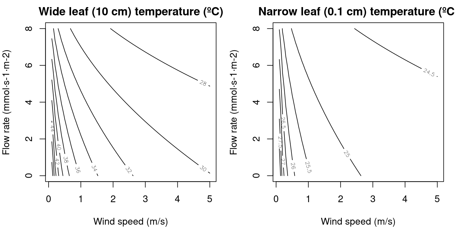
Figure 12.1: Values of $T_{leaf}$ for two leaf widths and varying values of wind speed and flow rate, calculated for 24ºC air temperature and 740 $W \cdot m^{-2}$ instantaneous absorbed radiation (including SWR and LWR).

Let us now fix wind speed at the leaf level to $u_{leaf} = 2$ m/s. The application of the leaf energy balance equation (11.1) to the $E(\Psi_{leaf})$ curves corresponding to the complete hydraulic network (10.4.5) yields the following $T_{leaf}(\Psi_{leaf})$ curves:

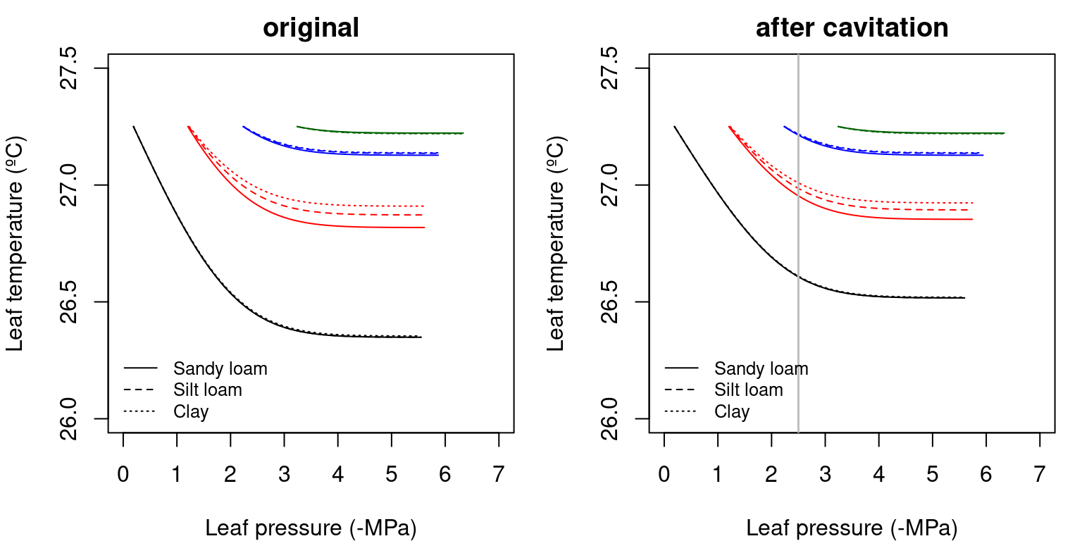
Figure 12.2: Examples of leaf temperature functions for a hydraulic network, corresponding to fig. 10.15 and for different soil textures. Left/right panel shows values for uncavitated/cavitated supply functions.

Leaf vapor deficit

Since $e_{leaf}$ decreases when leaf temperature decreases in eq. (11.4), increasing transpiration decreases leaf VPD as a result of decreasing leaf temperature. To illustrate this effect, let us assume the following values of relative humidity, yielding a $e_{air} = e_{atm} =1.91\, kPa$:

RHmin = 60
RHmax = 75
VPatm = meteoland::utils_averageDailyVP(Tmin, Tmax, RHmin, RHmax)
VPatm

## [1] 1.912181

The application of eqs. (11.3) and (11.4) to the $T_{leaf}(\Psi_{leaf})$ curves of fig. 12.2 yields the following $VPD_{leaf}(\Psi_{leaf})$ curves:

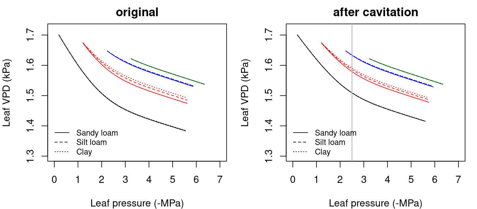
Figure 12.3: Examples of leaf vapour pressure deficit ($VPD_{leaf}$) functions for a hydraulic network, corresponding to fig. 10.15 and for different soil textures. Left/right panel shows values for uncavitated/cavitated supply functions.

Note that the VPD decreasing curves do not start at the same $VPD_{leaf}$ value despite corresponding to the same $T_{leaf}$ value, because of the effect of $\Psi_{leaf}$ on $e_{leaf}$ in eq. (11.4).

Stomatal conductance

The application of equations for $g_{w}$, $g_{bound}$ and $g_{sw}$ to the $VPD_{leaf}(\Psi_{leaf})$ curves yields the following stomatal conductance $g_{sw}(\Psi_{leaf})$ curves:

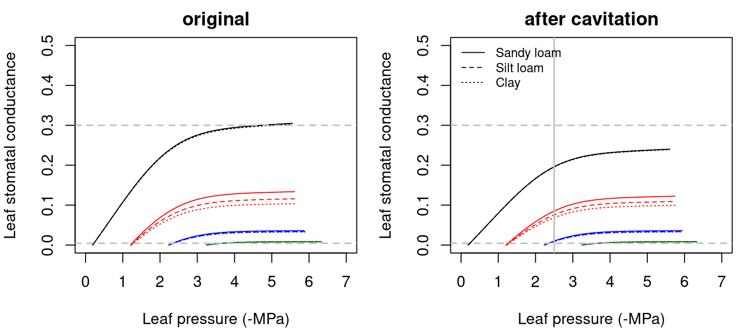
Figure 12.4: Examples of stomatal conductance to water vapor ($g_{sw}$) functions for a hydraulic network, corresponding to fig. 10.15 and for different soil textures. Left/right panel shows values for uncavitated/cavitated supply functions. Minimum and maximum conductance values ($g_{sw,\min} = 0.0045$ and $g_{sw,\max} = 0.3$) are indicated using dashed lines.

In the previous figure we have indicated the thresholds of $g_{sw,\min}$ and $g_{sw,\max}$, the species-specific minimum and maximum water vapour conductances (i.e. conductances when stomata are fully closed and fully open, respectively; see parameters Gswmin and Gswmax in SpParamsMED). $g_{sw}$ cannot exceed $g_{sw,\max}$ so that some flow rates may not be possible (see stomatal regulation below). However, $g_{sw,\max}$ should quickly become non-limiting as soil dries (i.e. reducing $E$) or $VPD_{leaf}$ increases (Sperry et al. 2017).

Leaf photosynthesis

Thus, after defining PAR photon flux density, canopy air $CO_{2}$ concentration and maximum rate parameters:

Q = 2000
Cair = 386
Vmax298 = 100
Jmax298 = 1.67*Vmax298

one can obtain the following $A(\Psi_{leaf})$ curves from $T_{leaf}(\Psi_{leaf})$ and $g_{sw}(\Psi_{leaf})$:

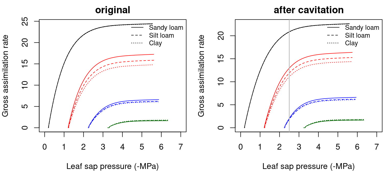
Figure 12.5: Examples of gross photosynthesis ($A$) functions for a hydraulic network, corresponding to fig. 10.15 and for different soil textures. Left/right panel shows values for uncavitated/cavitated supply functions.

Comparison of big-leaf, sun-shade and multi-canopy photosynthesis models

The figure below provides the canopy photosynthesis functions obtained using the multi-layer canopy photosynthesis model (top), a sunshade canopy photosynthesis model (center) or a big-leaf photosynthesis model (bottom). These were generated using functions photo_multilayerPhotosynthesisFunction(), photo_sunshadePhotosynthesisFunction() and photo_leafPhotosynthesisFunction(), respectively, and assuming homogeneous wind, temperature and water vapor pressure through the canopy. Thus, only absorbed radiation varied across layers and leaf types. Note the coincidence between the multi-layer and the sun-shade models.

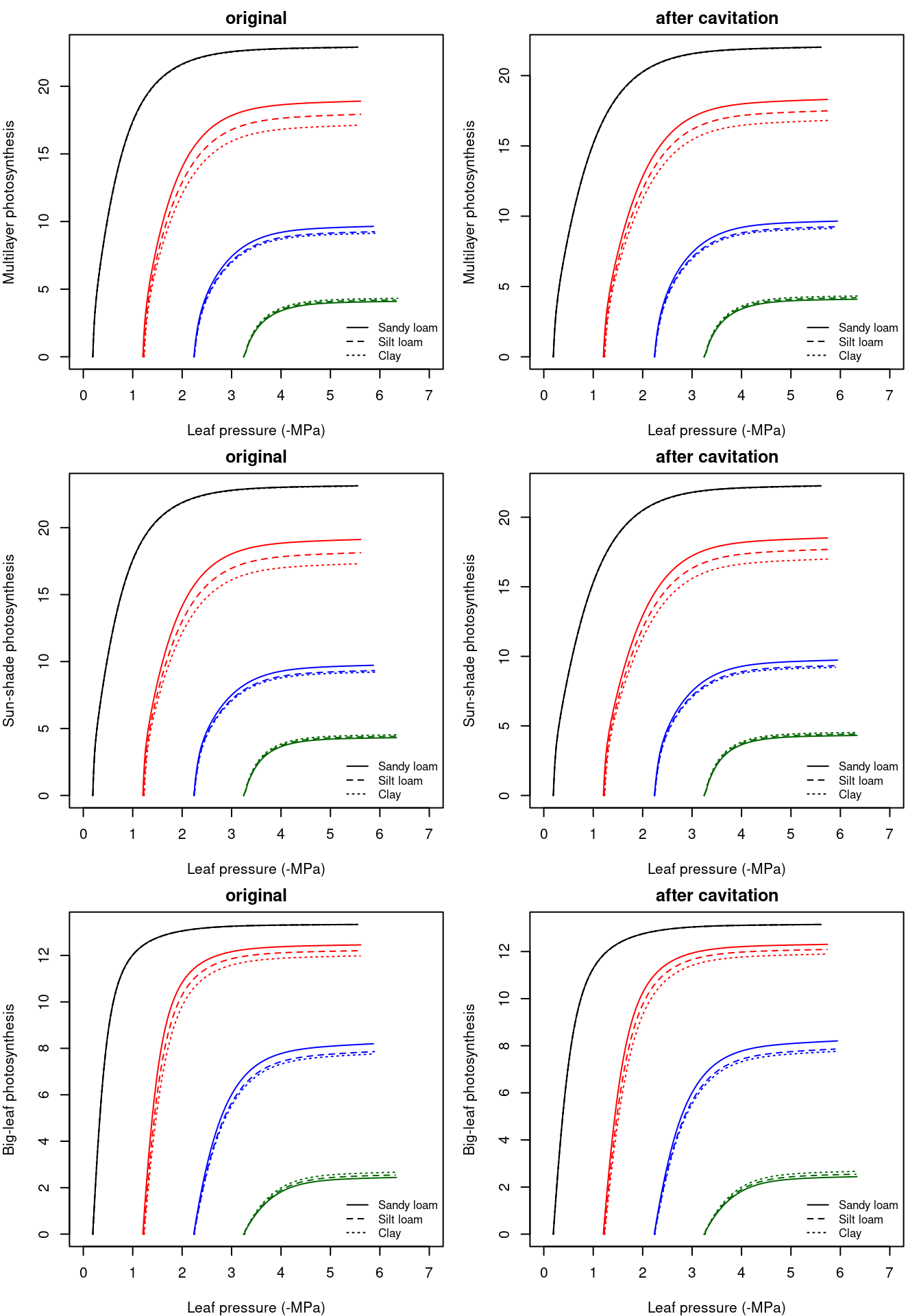
Figure 12.6: Whole-canopy photosynthesis functions obtained for a hydraulic network, corresponding to fig. 10.15 and different soil textures, using the multi-layer canopy photosynthesis model (top), a sunshade canopy photosynthesis model (center) or a big-leaf photosynthesis model (bottom). Left/right panel shows values for uncavitated/cavitated supply functions.

12.1.3 Leaf stomatal regulation by profit maximization

Wolf et al. (2016) proposed the carbon maximization criterion, which states that at each instant in time the stomata regulate canopy gas exchange and pressure to achieve the maximum profit, which is the maximum difference between photosynthetic gains and costs, the latter associated with hydraulic vulnerability attained with low water potentials. Such approach has been shown to be supported by data from global forest biomes (Anderegg et al. 2018). Building on this approach, Sperry et al. (2017) presented a profit maximization function where hydraulic costs of opening the stomata are compared against photosynthetic gains. Details of their formulation are given in this section. Stomatal regulation is performed in medfate separatedly for sunlit and shade leaves.

Cost and gain functions

The hydraulic supply function is used to derive a transpirational cost function $\theta_1(\Psi_{leaf})$ that reflects the increasing damage from cavitation and the greater difficulty of moving water along the continuum (Sperry et al. 2016): $$\begin{equation} \theta(\Psi_{leaf}) = \frac{k_{c,max}-k_{c}(\Psi_{leaf})}{k_{c,max}-k_{crit}} \end{equation}$$ where $k_c(\Psi_{leaf}) = dE/d\Psi(\Psi)$ is the slope of the supply function corresponding to (leaf) water potential $\Psi_{leaf}$, $k_{c,max}$ is the maximum slope of the supply function (which occurs when $E_{leaf}=0$), i.e. the maximum whole-plant conductance for the current soil moisture conditions, and $k_{crit} = k_c(\Psi_{crit})$ is the slope of the supply function at $E_{leaf} = E_{crit}$ the critical flow beyond which hydraulic failure occurs.

The following figures illustrate the $\theta(\Psi_{leaf})$ curves corresponding to the supply functions:

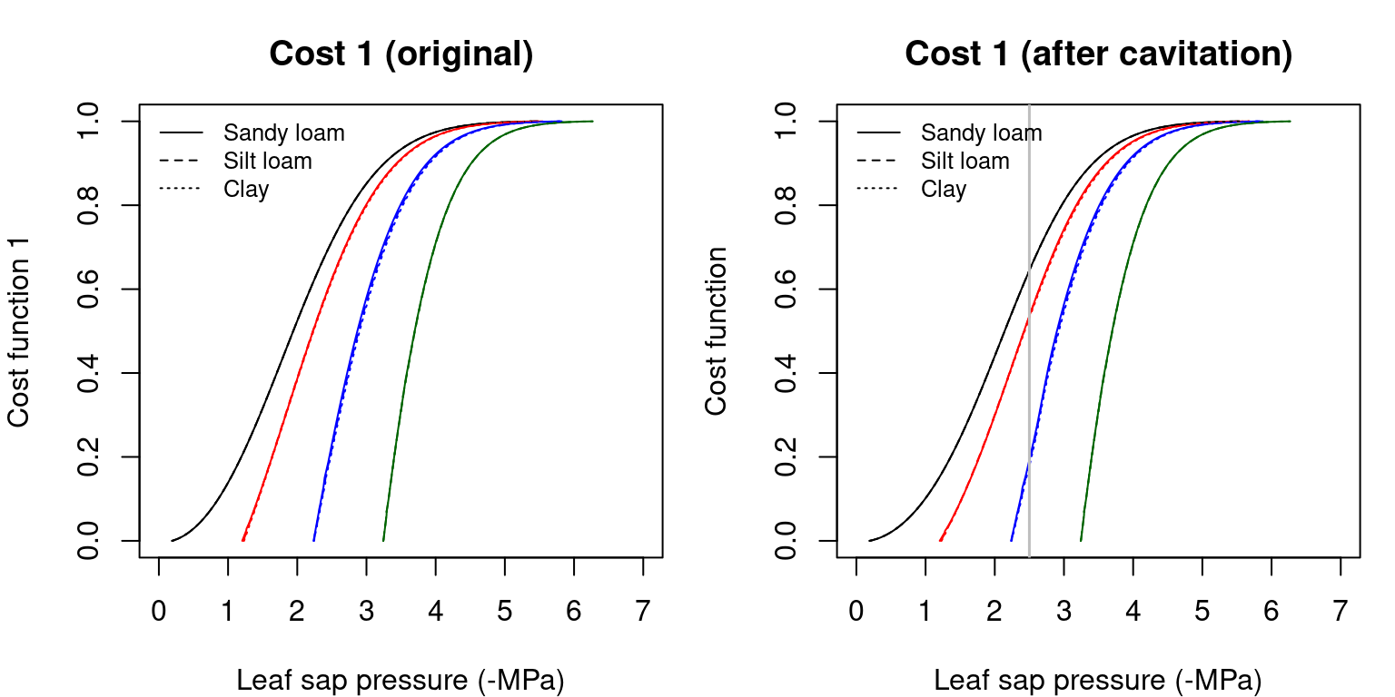
Figure 12.7: Cost functions (i.e. $\theta(\Psi_{leaf})$) obtained for a hydraulic network, corresponding to fig. 10.15 and different soil textures and soil water potentials. Left/right panels show values for uncavitated/cavitated supply functions, respectively.

The normalized photosynthetic gain function $\beta(\Psi_{leaf})$ reflects the actual assimilation rate with respect to the maximum (Sperry et al. 2016): $$\begin{equation} \beta(\Psi_{leaf}) = \frac{A(\Psi_{leaf})}{A_{max}} \end{equation}$$ where $A_{max}$ is the instantaneous maximum (gross) assimilation rate estimated over the full $\Psi_{leaf}$ range (including values that imply a stomatal conductance larger than the maximum).

The following figures illustrate the $\beta(\Psi_{leaf})$ curves corresponding to the supply and assimilation functions:

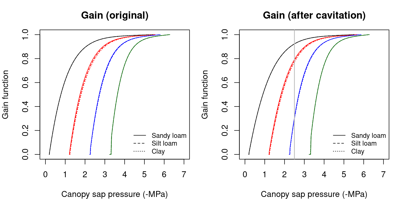
Figure 12.8: Gain function ($\beta(\Psi_{leaf})$) obtained for a hydraulic network, corresponding to fig. 10.15 and different soil textures and soil water potentials. Left/right panels show values for uncavitated/cavitated supply functions, respectively.

Profit maximization at the leaf level

Sperry et al. (2017) suggested that stomatal regulation can be effectively estimated by determining the maximum of the profit function ($Profit(\Psi_{leaf})$): $$\begin{equation} Profit(\Psi_{leaf}) = \beta(\Psi_{leaf})-\theta(\Psi_{leaf}) \end{equation}$$ The maximization is achieved when the slopes of the gain and cost functions are equal: $$\begin{equation} \frac{\delta \beta(\Psi_{leaf})}{\delta \Psi_{leaf}} = \frac{\delta \theta(\Psi_{leaf})}{\delta \Psi_{leaf}} \end{equation}$$ Instantaneous profit maximization assumes a ‘use it or lose it’ reality with regards to available soil water. Because the gain function accelerates more quickly from zero and reaches 1 sooner than the cost functiion, their maximum difference occurs at intermediate $\Psi_{leaf}$ values. Once $\Psi_{leaf}$ that maximizes profit is determined, the values of the remaining variables are also determined. At this point, it may happen that $g_{sw}(\Psi_{leaf})$ is lower than the minimum (i.e. cuticular) water vapor conductance ($g_{sw,\min}$) or larger than the maximum water vapor conductance ($g_{sw,\max}$). These thresholds need to be taken into account when determining the maximum of the profit function.

The following figures illustrate the $Profit(\Psi_{leaf})$ curves of corresponding to the previous cost and gain curves:

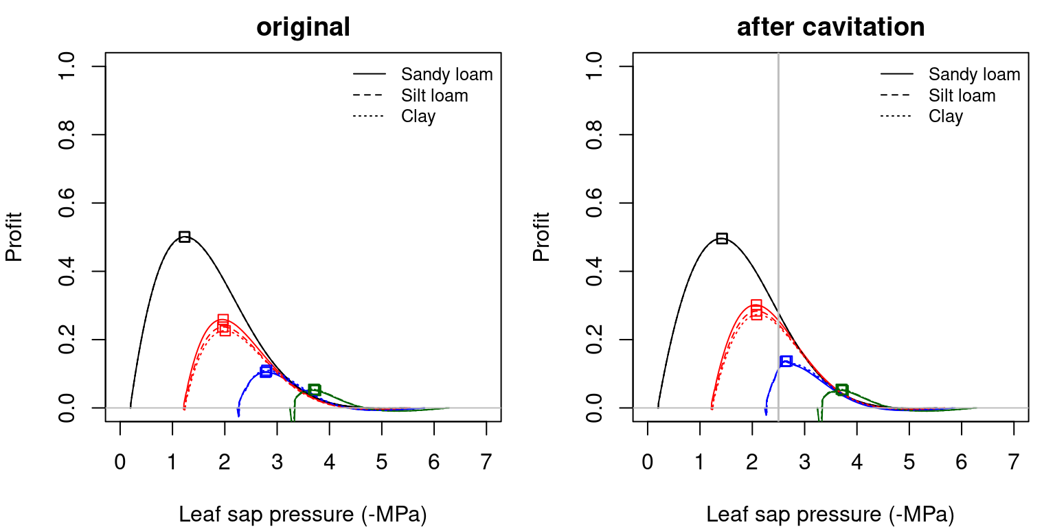
Figure 12.9: Profit functions (i.e. $Profit(\Psi_{leaf})$) obtained for a hydraulic network, corresponding to fig. 10.15 and different soil textures and soil water potentials. Left/right panels show values for uncavitated/cavitated supply functions, respectively.

Squares in the previous figures indicate the maximum profit points in each situation. The drier the soil, the closer is the maximum profit $\Psi_{leaf}$ to soil water potential as one would expect intuitively (i.e. a smaller drop in water potential along the hydraulic pathway). Note that when the soil is very dry the squares are to the right of the true maximum. This is because the transp_profitMaximization() function takes into account the minimum and maximum stomatal conductance and, in this case, does not allow optimum stomatal conductances below the minimum (cuticular) value.

Note that $\theta$, $\beta$ and $Profit$ functions can be expressed as a function of stomatal conductance, instead of leaf water potential. This allows visualizing more clearly the effect of $g_{sw,\min}$ and $g_{sw,\max}$ thresholds on the maximum profit optimization strategy, as illustrated in the following figures.

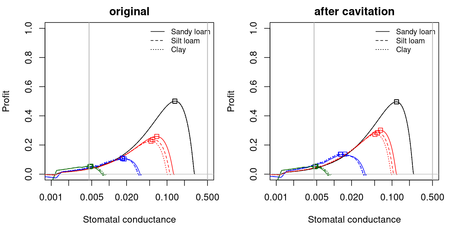
Figure 12.10: Profit function as a function of stomatal conductance, corresponding to fig. 12.9 and different soil textures and soil water potentials. Left/right panels show values for uncavitated/cavitated supply functions, respectively.

12.1.4 Plant-level transpiration rates and plant water potentials

In the previous section, we considered stomatal regulation at the level of sunlit or shade leaves only. At the plant cohort level, the gain function could be build from a crown photosynthesis function $A(\Psi_{leaf})$, as shown in section 11.2. However, applying the profit maximization approach for a single crown photosynthesis function would imply the assumption that the same stomatal aperture occurs in all leaves of the plant cohort, independently of whether they are in shade or sunlit. A more realistic approach is to determine stomatal regulation by profit maximization for sunlit and shade leaves separately. The gain function and profit maximization calculations conducted for each leaf type yield instantaneous leaf water potentials $\Psi^{sunlit}_{leaf}$ and $\Psi^{shade}_{leaf}$ and instantaneous flow values $E^{shade}$ and $E^{sunlit}$ from the supply functions. The corresponding photosynthesis functions allow determining values for leaf temperatures $T_{leaf}^{sunlit}$ and $T_{leaf}^{shade}$, vapor pressure deficits $VPD_{leaf}^{sunlit}$ $VPD_{leaf}^{shade}$, stomatal conductance $g_{sw}^{sunlit}$ and $g_{sw}^{shade}$ and net photosynthesis rates $A_{n}^{sunlit}$ and $A_{n}^{shade}$. This is a lot of useful information at the leaf level for each plant cohort, but we also need transpiration and photosynthesis values at the plant cohort-level.

The average instantaneous flow rate ($\hat{E}$, in $mmol\, H_2O \cdot s^{-1} \cdot m^{-2}$) per leaf area unit of a plant cohort is the weighed average: $$\begin{equation} \hat{E} = \frac{E^{shade} \cdot LAI^{sunlit} + E^{shade} \cdot LAI^{shade}}{LAI^{\phi}} \end{equation}$$ where $LAI^{sunlit}$ and $LAI^{shade}$ are the cohorts LAI values for sunlit and shade leaves, from eq. (9.1), and $LAI^{\phi}$ is the leaf area index of the plant cohort. The model then uses the hydraulic supply function to find the transpiration rate $E$ numerically closest to $\hat{E}$ (remember that the supply function is build in discrete steps). Finding the $E$ value numerically closest to $\hat{E}$ determines the $E_{plant}$, the instantaneous transpiration flow, and also leads to setting values for current time step of several other variables, such as water potentials ($\Psi_{leaf}$, $\Psi_{stem}$, $\Psi_{rootcrown}$, …), the slope of the supply function ($d E/d\Psi$), and instantaneous soil water uptake rates ($U_{s}$).

12.2 Stomatal regulation, transpiration and photosynthesis under Sureau’s sub-model

As mentioned in 7.5, with SurEau’s sub-model, leaf energy balance, stomatal and cuticular conductances, transpirational flows, photosynthesis and plant hydraulics are computed iteratively in small temporal sub-steps (e.g. 10 min). The following sections detail how leaf energy balance, conductances, transpiration and photosynthesis are estimated, whereas plant hydraulics were described in 10.5.

12.2.1 Transpiration flows

In Sureau-ECOS (Ruffault et al. 2022), plants lose water through stomatal transpiration ($E_{stom}$), cuticular transpiration of the leaf ($E_{leaf,cuti}$) and cuticular transpiration of the stem ($E_{stem, cuti}$), see Fig. 10.2. Therefore, the total plant transpiration $E_{plant}$ is decomposed as: $$\begin{equation} E_{plant} = E_{leaf} + E_{stem, cuti} = E_{stom} + E_{leaf, cuti} + E_{stem, cuti} \end{equation}$$ Since there are sunlit and shade, leaves, both $E_{stom}$ and $E_{leaf, cuti}$ are computed as weighted averages of sunlit and shade leaf values:

$$\begin{eqnarray} E_{stom} &=& \frac{E^{sunlit}_{stom} \cdot LAI^{sunlit} + E_{stom}^{shade} \cdot LAI^{shade}}{LAI^{\phi}} \\ E_{leaf,cuti} &=& \frac{E^{sunlit}_{leaf,cuti} \cdot LAI^{sunlit} + E_{leaf,cuti}^{shade} \cdot LAI^{shade}}{LAI^{\phi}} \end{eqnarray}$$

In turn, $E_{leaf,stom}^{sunlit}$, $E_{leaf,stom}^{shade}$, $E_{leaf,cuti}^{sunlit}$ and $E_{leaf,cuti}^{shade}$ values (all in $mmol\, H_2O \cdot s^{-1} \cdot m^{-2}$) are the result of multiplying the water vapor gradient by a compound conductance formed by either stomatal or cuticular conductances (which will likely be different for sunlit and shade leaves) and the leaf boundary layer conductance, i.e. (we ommit the sunlit/shade superscripts): $$\begin{eqnarray} E_{leaf, stom } &=& \left( g_{sw}^{-1} + g_{bound}^{-1} \right)^{-1} \cdot \frac{VPD_{leaf}}{P_{atm}} \\ E_{leaf, cuti} &=& \left( g_{leaf, cuti}^{-1} + g_{bound}^{-1} \right)^{-1} \cdot \frac{VPD_{leaf}}{P_{atm}} \end{eqnarray}$$

where $VPD_{leaf}$ (in MPa) is the vapor pressure deficit of the leaf (11.1.2), $P_{atm}$ is the atmospheric pressure, $g_{sw}$ is the stomatal conductance, $g_{leaf,cuti}$ is the cuticular conductance of the leaf and $g_{bound}$ is the conductance of the leaf boundary layer (here all in $mmol\, H_2O \cdot s^{-1} \cdot m^{-2}$). The overall transpiration rate of the leaf, $E_{leaf}$ has the following expression in the Fick’s law:

$$\begin{equation} E_{leaf} = g_{w} \cdot \frac{P_{atm}}{VPD_{leaf}} = \left( (g_{sw} + g_{cuti})^{-1} + g_{bound}^{-1} \right)^{-1} \cdot \frac{P_{atm}}{VPD_{leaf}} \end{equation}$$

Note that in Ruffault et al. (2022) a crown boundary conductance was also considered, but within the design of medfate it is not needed, since $VPD_{leaf}$ represents the gradient in vapor pressure between the leaf mesophyll and the canopy (or canopy layer) air.

Finally, $E_{stem, cuti}$ is calculated as follows: $$\begin{equation} E_{stem, cuti} = \left( g_{stem, cuti}^{-1} + g_{bound}^{-1} \right)^{-1} \cdot \frac{VPD_{air}}{P_{atm}} \end{equation}$$ where $VPD_{air}$ is the vapor pressure deficit in the canopy air, i.e.: $$\begin{equation} VPD_{air} = e_{sat}(T_{air}) - e_{air} \end{equation}$$

12.2.2 Cuticular conductances

Leaf cuticular conductances are not only species-specific, but can also change with temperature, according to changes in the permeability of lipid layers in the leaf epidermis. $g_{leaf,cuti}$ is a function of leaf temperature ($T_{leaf}$), which is based on a single or double Q10 equation depending on whether leaf temperature is above or below the transition phase temperature ($T_{phase}$). If $T_{leaf} \leq T_{phase}$ we have: $$\begin{equation} g_{leaf,cuti} = g_{leaf,cuti,20} \cdot Q_{10a}^{\frac{T_{leaf} - 20}{10}} \end{equation}$$ whereas if $T_{leaf} > T_{phase}$ we have: $$\begin{equation} g_{leaf,cuti} = g_{leaf,cuti,20} \cdot Q_{10a}^{\frac{T_{leaf} - 20}{10}} \cdot Q_{10b}^{\frac{T_{leaf} - T_{phase}}{10}} \end{equation}$$

Sunlit and shade leaves will have different $g_{leaf,cuti}$ because of their different temperature. Unlike $g_{leaf,cuti}$, $g_{stem, cuti}$ is assumed non temperature dependent.

12.2.3 Stomatal conductance

$g_{sw}$ is the stomatal conductance taking into account the dependence of stomata on light and temperature, as well as leaf water status, i.e:

$$\begin{equation} g_{sw} = \lambda(\Psi_{leaf,sym}) \cdot g_{sw, light, temp} \end{equation}$$

where $g_{sw, light, temp}$ is the stomatal conductance value without water stress, and $\lambda$ is a regulation factor that varies between 0 and 1 to represent stomatal closure according to leaf symplasmic water potential ($\Psi_{leaf,sym}$) using a sigmoid-type function:

$$\begin{equation} \lambda(\Psi_{leaf,sym}) = 1 - \left(1 + e^{(slope_{gs}/25) \cdot (\Psi_{leaf,sym} - \Psi50_{gs}}) \right)^{-1} \end{equation}$$

depending on the potential at 50 % of stomatal closure ($\Psi50_{gs}$) and a shape parameter ($slope_{gs}$) describing the rate of decrease in stomatal conductance per unit of water potential drop. With the current implementation, $\lambda$ will be the same for sunlit and shade leaves (i.e. there is only one symplasmic water potential for both kind of leaves) but $g_{sw, light, temp}$ will differ because of the different light and temperature conditions.

Stomatal regulation according to light and temperature can be performed following either a Jarvis (1976) or Baldocchi (1994), as dictated by the control parameter stomatalSubmodel (by default set to Baldocchi-type).

Jarvis-type stomatal regulation

In the Jarvis-type approach (Jarvis 1976), stomatal conductance according to light and temperature ($g_{sw, light, temp}$) is defined as:

$$\begin{equation} g_{sw, light, temp} = g_{sw, night, temp} + (g_{sw, max, temp} - g_{sw,night, temp}) \cdot (1 - e^{-Q_{PAR}^{leaf} \cdot c_{PAR}}) \end{equation}$$ where $g_{sw, max, temp}$ and $g_{sw, night, temp}$ are the maximum stomatal conductance and nocturnal stomatal conductance after accounting for temperature effects, $Q_{PAR}^{leaf}$ is the absorbed PAR photon flux per leaf area ((11.10)) and $c_{PAR}$ is an empirical coefficient. Temperature effects on maximum stomatal conductance are modelled using: $$\begin{equation} g_{sw, max, temp} = g_{sw, max} \cdot \left[ 1 + \left(\frac{T_{leaf} - T_{optim}}{T_{gs,sens}}\right)^2 \right]^{-1} \end{equation}$$ where $T_{leaf}$ is the current leaf temperature, $T_{optim}$ is the optimal temperature and $T_{gs, sens}$ is an empirical coefficient. Temperature effects on nocturnal stomatal conductance are modelled analogously.

Baldocchi-type stomatal regulation

Baldocchi (1994) presented an analytical solution of the coupled leaf photosyntesis and stomatal conductance models. Baldocchi’s approach uses Farquhar’s model to determine photosynthesis, and the stomatal conductance equation is: $$\begin{equation} g_{sw, light, temp} = g_{sw, 0} + m_{wue} \cdot \frac{A_n}{C_s} \end{equation}$$ where $m_{wue}$ is a dimensionless slope representing the water use efficiency, $A_n$ is net photosynthesis as determined by Farquhar’s model (which accounts for light and temperature effects), $g_{sw, 0}$ is the zero intercept when $A_{n} = 0$, here taken as $g_{sw,0} = g_{sw, night}$ and $C_{s}$ is the $CO_2$ concentration inside stomata, i.e.: $$\begin{equation} C_{s} = C_{air} - (A_{n}/g_{bc}) \end{equation}$$ where $C_{air}$ is the inside the canopy $CO_2$ concentration and $g_{bc}$ is the boundary layer for $CO_2$:

$$\begin{equation} g_{bc} = g_{bound}/1.6 \end{equation}$$

Note that $A_{n}$ is only calculated here to find the analytical solution to $g_{sw, light, temp}$. It does not represent actual photosynthesis, which has to be calculated taking into account leaf water status (i.e. $\lambda(\Psi_{leaf,sym})$). This is detailed in the next subsection.

12.2.4 Photosynthesis

Instantaneous gross and net photosynthesis rates for sunlit and shade leaves (i.e., $A_{g}^{shade}$, $A_{g}^{sunlit}$, $A_{n}^{shade}$, $A_{n}^{sunlit}$) are calculated using Farquhar’s model (11.1.4) and assuming that $g_{c}$, the leaf diffusive conductance for $CO_2$ is influenced by leaf boundary ($g_{bound}$), stomatal ($g_{sw}$) and leaf cuticular ($g_{leaf, cuti}$) conductances, as explained in 11.1.3. Hence, non-zero gross assimilation can still occur with stomata completely closed.

12.3 Scaling of transpiration, soil water uptake and photosynthesis rates

The amount of transpiration of a woody plant cohort in a given time step $t$ ($Tr_{woody, t}$, in $l \cdot m^{-2}$ of ground area, i.e. mm) is: $$\begin{equation} Tr_{woody,t} = E_{plant} \cdot LAI^{\phi} \cdot f_{dry} \cdot 10^{-3} \cdot 0.01802 \cdot \Delta t_{step} \tag{12.1} \end{equation}$$ where $E_{plant}$ is the instantaneous cohort-level transpiration rate ($mmol\,H_2O \cdot s^{-1} \cdot m^{-2}$ of leaf area), $0.01802$ is the molar weight (in $kg = l$) of water and $\Delta t_{step} = 86400/n_t$ the size of the time step in seconds, being $n_t$ the number of time steps. $f_{dry}$ is the fraction of the canopy that is assumed dry, which is necessary to avoid overestimating total evapo-transpiration. In non-rainy days $f_{dry} = 1$ whereas in rainy days it is derived from comparing the daily evaporation due to rainfall interception ($In$; in $mm$) with Penman’s potential evapo-transpiration ($PET$; in $mm$):

$$\begin{equation} f_{dry} = 1.0 - \frac{In}{PET} \end{equation}$$

Instantaneous water uptake rates from a given soil layer $s$ ($U_{s}$; in $mmol\,H_2O \cdot s^{-1} \cdot m^{-2}$ of leaf area) are scaled to the time step as done for transpiration: $$\begin{equation} Ex_{woody,s,t} = U_{s} \cdot LAI^{\phi} \cdot f_{dry} \cdot 10^{-3} \cdot 0.01802 \cdot \Delta t_{step} \tag{12.2} \end{equation}$$

Under the Sperry model, the sum of soil extraction equals transpiration, i.e.: $$\begin{equation} Tr_{woody,t} = Ex_{woody,t} = \sum_s {Ex_{woody,s,t}} \end{equation}$$ In contrast, under the SurEau model, soil extraction may not be equal to transpiration, leading to a change in plant water content (see (7.2)).

Instantaneous net photosynthesis per leaf area of sunlit and shade leaves in a given time step $t$ (i.e. $A_{n,t}^{sunlit}$ and $A_{n,t}^{shade}$) are also aggregated into $A_{n,t}$, the net photosynthesis of the plant cohort for the time step $t$, in $g\,C \cdot m^{-2}$ of ground area: $$\begin{equation} A_{n,t} = (A_{n,t}^{sunlit} \cdot LAI^{sunlit} + A_{n,t}^{shade} \cdot LAI^{shade}) \cdot 10^{-6} \cdot 12.01017 \cdot \Delta t_{step} \tag{12.3} \end{equation}$$ Scaling of gross photosynthesis rates is done analogously.

Bibliography

Anderegg, W.R.L., Wolf, A., Arango-Velez, A., Choat, B., Chmura, D.J., Jansen, S., et al. (2018). Woody plants optimise stomatal behaviour relative to hydraulic risk. Ecology Letters, 21, 968–977.

Baldocchi, D. (1994). An analytical solution for coupled leaf photosynthesis and stomatal conductance models. Tree Physiology, 14, 1069–1079.

Jarvis, P.G. (1976). The Interpretation of the variations in leaf water potential and stomatal conductance found in canopies in the field. Philosophical Transactions of the Royal Society B: Biological Sciences, 273, 593–610.

Ruffault, J., Pimont, F., Cochard, H., Dupuy, J.-L. & Martin-StPaul, N. (2022). SurEau-Ecos v2.0: A trait-based plant hydraulics model for simulations of plant water status and drought-induced mortality at the ecosystem level. Geoscientific Model Development, 15, 5593–5626.

Sperry, J.S., Adler, F.R., Campbell, G.S. & Comstock, J.P. (1998). Limitation of plant water use by rhizosphere and xylem conductance: Results from a model. Plant, Cell & Environment, 21, 347–359.

Sperry, J.S. & Love, D.M. (2015). What plant hydraulics can tell us about responses to climate-change droughts. New Phytologist, 207, 14–27.

Sperry, J.S., Venturas, M.D., Anderegg, W.R.L., Mencuccini, M., Mackay, D.S., Wang, Y., et al. (2017). Predicting stomatal responses to the environment from the optimization of photosynthetic gain and hydraulic cost. Plant, Cell & Environment, 40, 816–830.

Sperry, J.S., Wang, Y., Wolfe, B.T., Mackay, D.S., Anderegg, W.R.L., Mcdowell, N.G., et al. (2016). Pragmatic hydraulic theory predicts stomatal responses to climatic water deficits. New Phytologist, 212, 577–589.

Wolf, A., Anderegg, W.R.L. & Pacala, S.W. (2016). Optimal stomatal behavior with competition for water and risk of hydraulic impairment. Proceedings of the National Academy of Sciences, 113, E7222–E7230.